nullprogram.com/blog/2008/02/22/

I have gotten several e-mails lately about using GNU Octave. One
specifically was about blurring images in Octave. In response, I am
writing this in-depth post to cover spatial filters, and how to use
them in GNU Octave (a free implementation of the Matlab programming
language). This should be the sort of information you would find near
the beginning of an introductory digital image processing textbook,
but written out more simply. In the future, I will probably be writing
a post covering non-linear spatial and/or frequency domain filters in
Octave.
If you want to follow along in Octave, I strongly recommend that you
upgrade to the new Octave 3.0. It is considered stable, but differs
significantly from Octave 2.1, which many people may be used to. You
will also need to install
the image
processing package
from Octave-Forge. To get
help with any Octave function, just type help
<function>.
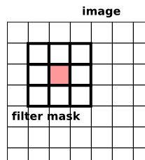
The most common linear spatial image filtering
involves
convolving a filter mask, sometimes called a convolution
kernel, over an image, which is a two-dimensional matrix. In the
case of an RGB color
image, the image is actually composed of three two-dimensional
grayscale images, each representing a single color, where each is
convolved with the filter mask separately.
Convolution is sliding a mask over an image. The new value at the
mask's position is the sum of the value of each element of the mask
multiplied by the value of the image at that position. For an example,
let's start with 1-dimensional convolution. Define a mask,
5 3 2 4 8
The 2 is the anchor for the mask. Define an image,
0 0 1 2 1 0 0
As we convolve, the mask will extend beyond the image at the
edges. One way to handle this is to pad the image with 0's. We start
by placing the mask at the left edge. (zero-padding is underlined)
Mask:   5 3 2 4 8
Image:  0 0 0 0 1 2 1 0 0
The first output value is 8, as every other element of the mask is
multiplied by zero.
Output: 8 x x x x x x
Now, slide the mask over by one position,
Mask:   5 3 2 4 8
Image:  0 0 0 1 2 1 0 0
The output here is 20, because 8*2 + 4*1 = 20;
Output: 8 20 x x x x x
If we continue sliding the mask along, the output becomes,
Output: 8 20 18 11 13 13 5
Here is the correlation done in Octave interactively,
(filter2() is the correlation function).
octave> filter2([5 3 2 4 8], [0 0 1 2 1 0 0])
ans =

    8   20   18   11   13   13    5
The same thing happens in two-dimensional convolution, with the mask
moving in the vertical direction as well, so that each element in the
image is covered.
Sometimes you will hear this described as correlation
(Octave's filter2) or convolution
(Octave's conv2). The only difference between these
operations is that in convolution the filter masked is rotated 180
degrees. Whoop-dee-doo. Most of the time your filter is probably
symmetrical anyway. So, don't worry much about the difference between
these two. Especially in Octave, where rotating a matrix is easy
(see rot90()).
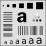
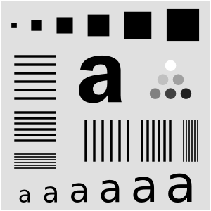
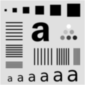
Now that we know convolution, let's introduce the sample image we will
be using. I carefully put this together
in Inkscape, which should give
us a nice scalable test image. When converting to a raster format,
there is a bit of unwanted anti-aliasing going on (couldn't find a way
to turn that off), but it is minimal.
Save that image (the PNG file, not the linked SVG file) where you can
get to it in Octave. Now, let's load the image into Octave
using imread().
m = imread("image-test.png");
The image is a grayscale image, so it has only one layer. The size
of m should be 300x300. You can check this like so (note
the lack of semicolon so we can see the output),
size(m)
You can view the image stored in m
with imshow. It doesn't care about the image dimensions
or size, so until you resize the plot window, it will probably be
stretched.
imshow(m);
Now, let's make an extremely simple 5x5 filter mask.
f = ones(5) * 1/25
Octave will show us what this matrix looks like.
f =

   0.040000   0.040000   0.040000   0.040000   0.040000
   0.040000   0.040000   0.040000   0.040000   0.040000
   0.040000   0.040000   0.040000   0.040000   0.040000
   0.040000   0.040000   0.040000   0.040000   0.040000
   0.040000   0.040000   0.040000   0.040000   0.040000
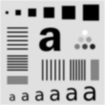
This filter mask is called an averaging filter. It simply
averages all the pixels around the image (think about how this works
out in the convolution). The effect will be to blur the image. It is
important to note here that the sum of the elements is 1 (or 100% if
you are thinking of averages). You can check it like so,
sum(f(:))
Now, to convolve the image with the filter mask
using filter2().
ave_m = filter2(f, m);
You can view the filtered image again with imshow()
except that we need to first convert the image matrix to a matrix of
8-bit unsigned integers. It is kind of annoying that we need this, but
this is the way it is as of this writing.
ave_m = uint8(ave_m);
imshow(ave_m);
Or, we can save this image to a file
using imwrite(). Just like with imshow(),
you will first need to convert the image to uint8.
imwrite("averaged.png", ave_m);
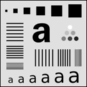
There are a few things to notice about this image. First there is a
black border around the outside of the filtered image. This is due to
the zero-padding (black border) done by filter2(). The
border of the image had 0's averaged into them. Second, some parts of
the blurred image are "noisy". Here are some selected parts at 4x zoom.
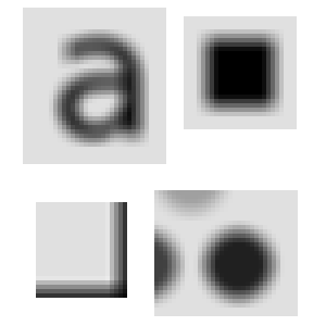
Notice how the circle, and the "a" seem a little bit boxy? This is due
to the shape of our filter. Also notice that the blurring isn't as
smooth as it could be. This is because the filter itself isn't very
smooth. We'll fix both these problems with a new filter later.
First, here is how we can fix the border problem: we pad the image
with itself. Octave provides us three easy ways to do this. The first
is replicate padding: the padding outside the image is the same as the
nearest border pixel in the image. Circular padding: the padding from
from the opposite side of the image, as if it was wrapped. This would
be a good choice for a periodic image. Last, and probably the most
useful is symmetric: the padding is a mirror reflection of the image
itself.
To apply symmetric padding, we use the padarray()
function. We only want to pad the image by the amount that the mask
will "hang off". Let's pad the original image for a 9x9 filter, which
will hang off by 4 pixels each way,
mpad = padarray(m, [4 4], "symmetric");
Next, we will replace the averaging filter with a 2D Gaussian
distribution. The Gaussian, or normal, distribution has many wonderful
and useful properties (as a statistics professor I had once said,
anyone who considers themselves to be educated should know about the
normal distribution). One property that makes it useful is that if we
integrate the Gaussian distribution from minus infinity to infinity,
the result is 1. The easiest way to get the curve without having to
type in the equation is using fspecial(): a special
function for creating image filters.
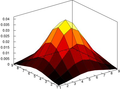
f_gauss = fspecial("gaussian", 9, 2);
This creates a 9x9 Gaussian filter with variance 2. The variance
controls the effective size of the filter. Increasing the size of the
filter from 9 to 99 will actually have virtually no impact on the
final result. It just needs to be large enough to cover the curve. Six
times the variance covers over 99% of the curve, so for a variance of
2, a filter of size 7x7 (always make your filters odd in size) is
plenty. A larger filter means a longer convolution time. Here is what
the 9x9 filter looks like,
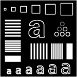
And to filter with the Gaussian,
gauss_m = filter2(f_gauss, mpad, "valid";
gauss_m = uint8(guass_m);
Notice the extra argument "valid"? Since we padded the
image before filtering, we don't want this padding to be part of the
image result. filter2() normally returns an image of the
same size as the input image, but we only want the part that didn't
undergo (additional) zero-padding. The result is now the same size as
the original image, but without the messy border,
Also, compare the result to the average filter above. See how much
smoother this image is? If you are interested in blurring an image,
you will generally want to go with a Gaussian filter like this.
Now I will let you in on a little shortcut. In Matlab, there is a
function called imfilter which does the padding and
filtering in one step. As of this writing, the Octave-Forge image
package doesn't officially include this function, but it is there in
the source repository now, meaning that it will probably appear in the
next version of that package. I actually wrote my own before I found
this one. You can grab the official one
here:
imfilter.m
With this new function, we can filter with the Gaussian and save like
this. Notice the flipping of the first two arguments
from filter2, as well as the lack of converting
to uint8.
gauss_m = imfilter(m, f, "symmetric");
imwrite("gauss.png", gauss_m);
imfilter() will also handle the 3-layer color images
seamlessly. Without it, you would need to run filter2()
on each layer separately.
So that is just about all there is. fspecial() has many
more filters available including motion
blur,
unsharp, and edge detection. For example,
the Sobel edge
detector,
octave:25> fspecial("sobel")
ans =

   1   2   1
   0   0   0
  -1  -2  -1
It is good at detecting edges in one direction. We can rotate this
each way to detect edges all over the image.
mf = uint8(zeros(size(m)));
for i = 0:3
  mf += imfilter(m, rot90(fspecial("sobel"), i));
end
imshow(mf)

Happy Hacking with Octave!