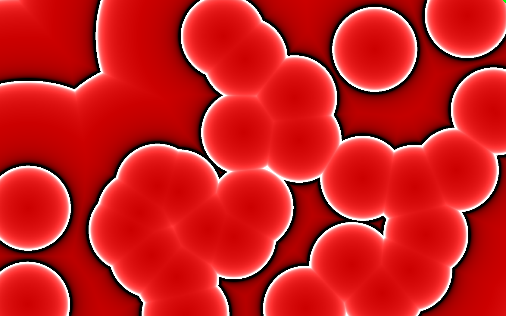
It’s interactive. The mouse cursor is a circular obstacle that the particles bounce off of, and clicking will place a permanent obstacle in the simulation. You can paint and draw structures through which the the particles will flow.
Here’s an HTML5 video of the demo in action, which, out of necessity, is recorded at 60 frames-per-second and a high bitrate, so it’s pretty big. Video codecs don’t gracefully handle all these full-screen particles very well and lower framerates really don’t capture the effect properly. I also added some appropriate sound that you won’t hear in the actual demo.
On a modern GPU, it can simulate and draw over 4 million particles at 60 frames per second. Keep in mind that this is a JavaScript application, I haven’t really spent time optimizing the shaders, and it’s living within the constraints of WebGL rather than something more suitable for general computation, like OpenCL or at least desktop OpenGL.
Just as with the Game of Life and path finding projects, simulation state is stored in pairs of textures and the majority of the work is done by a fragment shader mapped between them pixel-to-pixel. I won’t repeat myself with the details of setting this up, so refer to the Game of Life article if you need to see how it works.
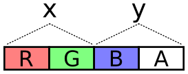
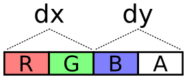
For this simulation, there are four of these textures instead of two: a pair of position textures and a pair of velocity textures. Why pairs of textures? There are 4 channels, so every one of these components (x, y, dx, dy) could be packed into its own color channel. This seems like the simplest solution.
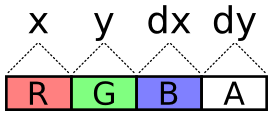
The problem with this scheme is the lack of precision. With the R8G8B8A8 internal texture format, each channel is one byte. That’s 256 total possible values. The display area is 800 by 600 pixels, so not even every position on the display would be possible. Fortunately, two bytes, for a total of 65,536 values, is plenty for our purposes.
The next problem is how to encode values across these two channels. It needs to cover negative values (negative velocity) and it should try to take full advantage of dynamic range, i.e. try to spread usage across all of those 65,536 values.
To encode a value, multiply the value by a scalar to stretch it over the encoding’s dynamic range. The scalar is selected so that the required highest values (the dimensions of the display) are the highest values of the encoding.
Next, add half the dynamic range to the scaled value. This converts
all negative values into positive values with 0 representing the
lowest value. This representation is called Excess-K. The
downside to this is that clearing the texture (glClearColor
) with
transparent black no longer sets the decoded values to 0.
Finally, treat each channel as a digit of a base-256 number. The OpenGL ES 2.0 shader language has no bitwise operators, so this is done with plain old division and modulus. I made an encoder and decoder in both JavaScript and GLSL. JavaScript needs it to write the initial values and, for debugging purposes, so that it can read back particle positions.
vec2 encode(float value) {
value = value * scale + OFFSET;
float x = mod(value, BASE);
float y = floor(value / BASE);
return vec2(x, y) / BASE;
}
float decode(vec2 channels) {
return (dot(channels, vec2(BASE, BASE * BASE)) - OFFSET) / scale;
}
And JavaScript. Unlike normalized GLSL values above (0.0-1.0), this produces one-byte integers (0-255) for packing into typed arrays.
function encode(value, scale) {
var b = Particles.BASE;
value = value * scale + b * b / 2;
var pair = [
Math.floor((value % b) / b * 255),
Math.floor(Math.floor(value / b) / b * 255)
];
return pair;
}
function decode(pair, scale) {
var b = Particles.BASE;
return (((pair[0] / 255) * b +
(pair[1] / 255) * b * b) - b * b / 2) / scale;
}
The fragment shader that updates each particle samples the position
and velocity textures at that particle’s “index”, decodes their
values, operates on them, then encodes them back into a color for
writing to the output texture. Since I’m using WebGL, which lacks
multiple rendering targets (despite having support for gl_FragData
),
the fragment shader can only output one color. Position is updated in
one pass and velocity in another as two separate draws. The buffers
are not swapped until after both passes are done, so the velocity
shader (intentionally) doesn’t uses the updated position values.
There’s a limit to the maximum texture size, typically 8,192 or 4,096, so rather than lay the particles out in a one-dimensional texture, the texture is kept square. Particles are indexed by two-dimensional coordinates.
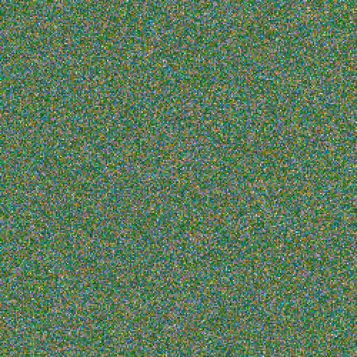
It’s pretty interesting to see the position or velocity textures drawn directly to the screen rather than the normal display. It’s another domain through which to view the simulation, and it even helped me identify some issues that were otherwise hard to see. The output is a shimmering array of color, but with definite patterns, revealing a lot about the entropy (or lack thereof) of the system. I’d share a video of it, but it would be even more impractical to encode than the normal display. Here are screenshots instead: position, then velocity. The alpha component is not captured here.
One of the biggest challenges with running a simulation like this on a
GPU is the lack of random values. There’s no rand()
function in the
shader language, so the whole thing is deterministic by default. All
entropy comes from the initial texture state filled by the CPU. When
particles clump up and match state, perhaps from flowing together over
an obstacle, it can be difficult to work them back apart since the
simulation handles them identically.
To mitigate this problem, the first rule is to conserve entropy whenever possible. When a particle falls out of the bottom of the display, it’s “reset” by moving it back to the top. If this is done by setting the particle’s Y value to 0, then information is destroyed. This must be avoided! Particles below the bottom edge of the display tend to have slightly different Y values, despite exiting during the same iteration. Instead of resetting to 0, a constant value is added: the height of the display. The Y values remain different, so these particles are more likely to follow different routes when bumping into obstacles.
The next technique I used is to supply a single fresh random value via a uniform for each iteration This value is added to the position and velocity of reset particles. The same value is used for all particles for that particular iteration, so this doesn’t help with overlapping particles, but it does help to break apart “streams”. These are clearly-visible lines of particles all following the same path. Each exits the bottom of the display on a different iteration, so the random value separates them slightly. Ultimately this stirs in a few bits of fresh entropy into the simulation on each iteration.
Alternatively, a texture containing random values could be supplied to the shader. The CPU would have to frequently fill and upload the texture, plus there’s the issue of choosing where to sample the texture, itself requiring a random value.
Finally, to deal with particles that have exactly overlapped, the particle’s unique two-dimensional index is scaled and added to the position and velocity when resetting, teasing them apart. The random value’s sign is multiplied by the index to avoid bias in any particular direction.
To see all this in action in the demo, make a big bowl to capture all the particles, getting them to flow into a single point. This removes all entropy from the system. Now clear the obstacles. They’ll all fall down in a single, tight clump. It will still be somewhat clumped when resetting at the top, but you’ll see them spraying apart a little bit (particle indexes being added). These will exit the bottom at slightly different times, so the random value plays its part to work them apart even more. After a few rounds, the particles should be pretty evenly spread again.
The last source of entropy is your mouse. When you move it through the scene you disturb particles and introduce some noise to the simulation.
This project idea occurred to me while reading the OpenGL ES shader language specification (PDF). I’d been wanting to do a particle system, but I was stuck on the problem how to draw the particles. The texture data representing positions needs to somehow be fed back into the pipeline as vertices. Normally a buffer texture — a texture backed by an array buffer — or a pixel buffer object — asynchronous texture data copying — might be used for this, but WebGL has none these features. Pulling texture data off the GPU and putting it all back on as an array buffer on each frame is out of the question.
However, I came up with a cool technique that’s better than both those
anyway. The shader function texture2D
is used to sample a pixel in a
texture. Normally this is used by the fragment shader as part of the
process of computing a color for a pixel. But the shader language
specification mentions that texture2D
is available in vertex
shaders, too. That’s when it hit me. The vertex shader itself can
perform the conversion from texture to vertices.
It works by passing the previously-mentioned two-dimensional particle
indexes as the vertex attributes, using them to look up particle
positions from within the vertex shader. The shader would run in
GL_POINTS
mode, emitting point sprites. Here’s the abridged version,
attribute vec2 index;
uniform sampler2D positions;
uniform vec2 statesize;
uniform vec2 worldsize;
uniform float size;
// float decode(vec2) { ...
void main() {
vec4 psample = texture2D(positions, index / statesize);
vec2 p = vec2(decode(psample.rg), decode(psample.ba));
gl_Position = vec4(p / worldsize * 2.0 - 1.0, 0, 1);
gl_PointSize = size;
}
The real version also samples the velocity since it modulates the color (slow moving particles are lighter than fast moving particles).
However, there’s a catch: implementations are allowed to limit the
number of vertex shader texture bindings to 0
(GL_MAX_VERTEX_TEXTURE_IMAGE_UNITS
). So technically vertex shaders
must always support texture2D
, but they’re not required to support
actually having textures. It’s sort of like food service on an
airplane that doesn’t carry passengers. These platforms don’t support
this technique. So far I’ve only had this problem on some mobile
devices.
Outside of the lack of support by some platforms, this allows every part of the simulation to stay on the GPU and paves the way for a pure GPU particle system.
An important observation is that particles do not interact with each other. This is not an n-body simulation. They do, however, interact with the rest of the world: they bounce intuitively off those static circles. This environment is represented by another texture, one that’s not updated during normal iteration. I call this the obstacle texture.
The colors on the obstacle texture are surface normals. That is, each pixel has a direction to it, a flow directing particles in some direction. Empty space has a special normal value of (0, 0). This is not normalized (doesn’t have a length of 1), so it’s an out-of-band value that has no effect on particles.
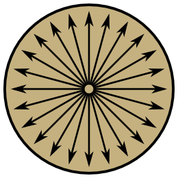
(I didn’t realize until I was done how much this looks like the Greendale Community College flag.)
A particle checks for a collision simply by sampling the obstacle
texture. If it finds a normal at its location, it changes its velocity
using the shader function reflect
. This function is normally used
for reflecting light in a 3D scene, but it works equally well for
slow-moving particles. The effect is that particles bounce off the the
circle in a natural way.
Sometimes particles end up on/in an obstacle with a low or zero velocity. To dislodge these they’re given a little nudge in the direction of the normal, pushing them away from the obstacle. You’ll see this on slopes where slow particles jiggle their way down to freedom like jumping beans.
To make the obstacle texture user-friendly, the actual geometry is maintained on the CPU side of things in JavaScript. It keeps a list of these circles and, on updates, redraws the obstacle texture from this list. This happens, for example, every time you move your mouse on the screen, providing a moving obstacle. The texture provides shader-friendly access to the geometry. Two representations for two purposes.
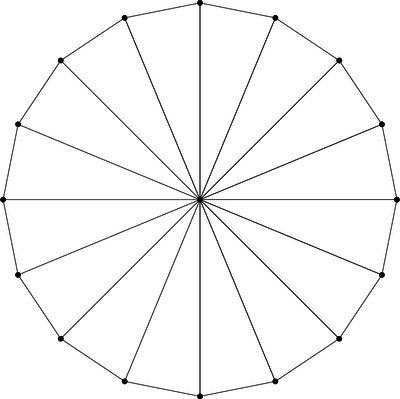
When I started writing this part of the program, I envisioned that shapes other than circles could place placed, too. For example, solid rectangles: the normals would look something like this.
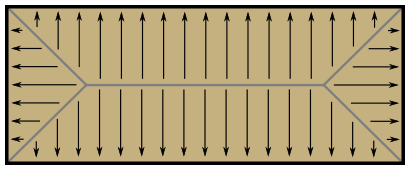
So far these are unimplemented.
I didn’t try it yet, but I wonder if particles could interact with each other by also drawing themselves onto the obstacles texture. Two nearby particles would bounce off each other. Perhaps the entire liquid demo could run on the GPU like this. If I’m imagining it correctly, particles would gain volume and obstacles forming bowl shapes would fill up rather than concentrate particles into a single point.
I think there’s still some more to explore with this project.
]]>The JavaScript side of things is essentially the same as before — two textures with fragment shader in between that steps the automaton forward — so I won’t be repeating myself. The only parts that have changed are the cell state encoding (to express all automaton states) and the fragment shader (to code the new rules).
Included is a pure JavaScript implementation of the cellular automaton (State.js) that I used for debugging and experimentation, but it doesn’t actually get used in the demo. A fragment shader (12state.frag) encodes the full automaton rules for the GPU.
There’s a dead simple 2-state cellular automaton that can solve any perfect maze of arbitrary dimension. Each cell is either OPEN or a WALL, only 4-connected neighbors are considered, and there’s only one rule: if an OPEN cell has only one OPEN neighbor, it becomes a WALL.
On each step the dead ends collapse towards the solution. In the above GIF, in order to keep the start and finish from collapsing, I’ve added a third state (red) that holds them open. On a GPU, you’d have to do as many draws as the length of the longest dead end.
A perfect maze is a maze where there is exactly one solution. This technique doesn’t work for mazes with multiple solutions, loops, or open spaces. The extra solutions won’t collapse into one, let alone the shortest one.
To fix this we need a more advanced cellular automaton.
I came up with a 12-state cellular automaton that can not only solve mazes, but will specifically find the shortest path. Like above, it only considers 4-connected neighbors.
If we wanted to consider 8-connected neighbors, everything would be the same, but it would require 20 states (n, ne, e, se, s, sw, w, nw) instead of 12. The rules are still pretty simple.
This can be generalized for cellular grids of any arbitrary dimension, and it could even run on a GPU for higher dimensions, limited primarily by the number of texture uniform bindings (2D needs 1 texture binding, 3D needs 2 texture bindings, 4D needs 8 texture bindings … I think). But if you need to find the shortest path along a five-dimensional grid, I’d like to know why!
So what does it look like?
FLOW cells flood the entire maze. Branches of the maze are search in parallel as they’re discovered. As soon as an END cell is touched, a ROUTE is traced backwards along the flow to the BEGIN cell. It requires double the number of steps as the length of the shortest path.
Note that the FLOW cell keep flooding the maze even after the END was found. It’s a cellular automaton, so there’s no way to communicate to these other cells that the solution was discovered. However, when running on a GPU this wouldn’t matter anyway. There’s no bailing out early before all the fragment shaders have run.
What’s great about this is that we’re not limited to mazes whatsoever. Here’s a path through a few connected rooms with open space.
The worst-case solution is the longest possible shortest path. There’s only one frontier and running the entire automaton to push it forward by one cell is inefficient, even for a GPU.
The way a maze is generated plays a large role in how quickly the cellular automaton can solve it. A common maze generation algorithm is a random depth-first search (DFS). The entire maze starts out entirely walled in and the algorithm wanders around at random plowing down walls, but never breaking into open space. When it comes to a dead end, it unwinds looking for new walls to knock down. This methods tends towards long, winding paths with a low branching factor.
The mazes you see in the demo are Kruskal’s algorithm mazes. Walls are knocked out at random anywhere in the maze, without breaking the perfect maze rule. It has a much higher branching factor and makes for a much more interesting demo.
On my computers, with a 1023x1023 Kruskal maze it’s about an
order of magnitude slower (see update below) than A*
(rot.js’s version) for the same maze. Not very
impressive! I believe this gap will close with time, as GPUs
become parallel faster than CPUs get faster. However, there’s
something important to consider: it’s not only solving the shortest
path between source and goal, it’s finding the shortest path between
the source and any other point. At its core it’s a breadth-first
grid search.
Update: One day after writing this article I realized that
glReadPixels
was causing a gigantic bottlebeck. By only checking for
the end conditions once every 500 iterations, this method is now
equally fast as A* on modern graphics cards, despite taking up to an
extra 499 iterations. In just a few more years, this technique
should be faster than A*.
Really, there’s little use in ROUTE step. It’s a poor fit for the GPU. It has no use in any real application. I’m using it here mainly for demonstration purposes. If dropped, the cellular automaton would become 6 states: OPEN, WALL, and four flavors of FLOW. Seed the source point with a FLOW cell (arbitrary direction) and run the automaton until all of the OPEN cells are gone.
The ROUTE cells do have a useful purpose, though. How do we know when we’re done? We can poll the BEGIN cell to check for when it becomes a ROUTE cell. Then we know we’ve found the solution. This doesn’t necessarily mean all of the FLOW cells have finished propagating, though, especially in the case of a DFS-maze.
In a CPU-based solution, I’d keep a counter and increment it every
time an OPEN cell changes state. The the counter doesn’t change after
an iteration, I’m done. OpenGL 4.2 introduces an atomic
counter that could serve this role, but this isn’t available in
OpenGL ES / WebGL. The only thing left to do is use glReadPixels
to
pull down the entire thing and check for end state on the CPU.
The original 2-state automaton above also suffers from this problem.
Cells are stored per pixel in a GPU texture. I spent quite some time trying to brainstorm a clever way to encode the twelve cell states into a vec4 color. Perhaps there’s some way to exploit blending to update cell states, or make use of some other kind of built-in pixel math. I couldn’t think of anything better than a straight-forward encoding of 0 to 11 into a single color channel (red in my case).
int state(vec2 offset) {
vec2 coord = (gl_FragCoord.xy + offset) / scale;
vec4 color = texture2D(maze, coord);
return int(color.r * 11.0 + 0.5);
}
This leaves three untouched channels for other useful information. I
experimented (uncommitted) with writing distance in the green channel.
When an OPEN cell becomes a FLOW cell, it adds 1 to its adjacent FLOW
cell distance. I imagine this could be really useful in a real
application: put your map on the GPU, run the cellular automaton a
sufficient number of times, pull the map back off (glReadPixels
),
and for every point you know both the path and total distance to the
source point.
As mentioned above, I ran the GPU maze-solver against A* to test its performance. I didn’t yet try running it against Dijkstra’s algorithm on a CPU over the entire grid (one source, many destinations). If I had to guess, I’d bet the GPU would come out on top for grids with a high branching factor (open spaces, etc.) so that its parallelism is most effectively exploited, but Dijkstra’s algorithm would win in all other cases.
Overall this is more of a proof of concept than a practical application. It’s proof that we can trick OpenGL into solving mazes for us!
]]>Conway’s Game of Life is another well-matched workload for GPUs. Here’s the actual WebGL demo if you want to check it out before continuing.
To quickly summarize the rules:
These simple cellular automata rules lead to surprisingly complex, organic patterns. Cells are updated in parallel, so it’s generally implemented using two separate buffers. This makes it a perfect candidate for an OpenGL fragment shader.
The entire simulation state will be stored in a single, 2D texture in GPU memory. Each pixel of the texture represents one Life cell. The texture will have the internal format GL_RGBA. That is, each pixel will have a red, green, blue, and alpha channel. This texture is not drawn directly to the screen, so how exactly these channels are used is mostly unimportant. It’s merely a simulation data structure. This is because I’m using the OpenGL programmable pipeline for general computation. I’m calling this the “front” texture.
Four multi-bit (actual width is up to the GPU) channels seems excessive considering that all I really need is a single bit of state for each cell. However, due to framebuffer completion rules, in order to draw onto this texture it must be GL_RGBA. I could pack more than one cell into one texture pixel, but this would reduce parallelism: the shader will run once per pixel, not once per cell.
Because cells are updated in parallel, this texture can’t be modified in-place. It would overwrite important state. In order to do any real work I need a second texture to store the update. This is the “back” texture. After the update, this back texture will hold the current simulation state, so the names of the front and back texture are swapped. The front texture always holds the current state, with the back texture acting as a workspace.
GOL.prototype.swap = function() {
var tmp = this.textures.front;
this.textures.front = this.textures.back;
this.textures.back = tmp;
return this;
};
Here’s how a texture is created and prepared. It’s wrapped in a function/method because I’ll need two identical textures, making two separate calls to this function. All of these settings are required for framebuffer completion (explained later).
GOL.prototype.texture = function() {
var gl = this.gl;
var tex = gl.createTexture();
gl.bindTexture(gl.TEXTURE_2D, tex);
gl.texParameteri(gl.TEXTURE_2D, gl.TEXTURE_WRAP_S, gl.REPEAT);
gl.texParameteri(gl.TEXTURE_2D, gl.TEXTURE_WRAP_T, gl.REPEAT);
gl.texParameteri(gl.TEXTURE_2D, gl.TEXTURE_MIN_FILTER, gl.NEAREST);
gl.texParameteri(gl.TEXTURE_2D, gl.TEXTURE_MAG_FILTER, gl.NEAREST);
gl.texImage2D(gl.TEXTURE_2D, 0, gl.RGBA,
this.statesize.x, this.statesize.y,
0, gl.RGBA, gl.UNSIGNED_BYTE, null);
return tex;
};
A texture wrap of GL_REPEAT
means the simulation will be
automatically torus-shaped. The interpolation is
GL_NEAREST
, because I don’t want to interpolate between cell states
at all. The final OpenGL call initializes the texture size
(this.statesize
). This size is different than the size of the
display because, again, this is actually a simulation data structure
for my purposes.
The null
at the end would normally be texture data. I don’t need to
supply any data at this point, so this is left blank. Normally this
would leave the texture content in an undefined state, but for
security purposes, WebGL will automatically ensure that it’s zeroed.
Otherwise there’s a chance that sensitive data might leak from another
WebGL instance on another page or, worse, from another process using
OpenGL. I’ll make a similar call again later with glTexSubImage2D()
to fill the texture with initial random state.
In OpenGL ES, and therefore WebGL, wrapped (GL_REPEAT
) texture
dimensions must be powers of two, i.e. 512x512, 256x1024, etc. Since I
want to exploit the built-in texture wrapping, I’ve decided to
constrain my simulation state size to powers of two. If I manually did
the wrapping in the fragment shader, I could make the simulation state
any size I wanted.
A framebuffer is the target of the current glClear()
,
glDrawArrays()
, or glDrawElements()
. The user’s display is the
default framebuffer. New framebuffers can be created and used as
drawing targets in place of the default framebuffer. This is how
things are drawn off-screen without effecting the display.
A framebuffer by itself is nothing but an empty frame. It needs a canvas. Other resources are attached in order to make use of it. For the simulation I want to draw onto the back buffer, so I attach this to a framebuffer. If this framebuffer is bound at the time of the draw call, the output goes onto the texture. This is really powerful because this texture can be used as an input for another draw command, which is exactly what I’ll be doing later.
Here’s what making a single step of the simulation looks like.
GOL.prototype.step = function() {
var gl = this.gl;
gl.bindFramebuffer(gl.FRAMEBUFFER, this.framebuffers.step);
gl.framebufferTexture2D(gl.FRAMEBUFFER, gl.COLOR_ATTACHMENT0,
gl.TEXTURE_2D, this.textures.back, 0);
gl.viewport(0, 0, this.statesize.x, this.statesize.y);
gl.bindTexture(gl.TEXTURE_2D, this.textures.front);
this.programs.gol.use()
.attrib('quad', this.buffers.quad, 2)
.uniform('state', 0, true)
.uniform('scale', this.statesize)
.draw(gl.TRIANGLE_STRIP, 4);
this.swap();
return this;
};
First, bind the custom framebuffer as the current framebuffer with
glBindFramebuffer()
. This framebuffer was previously created with
glCreateFramebuffer()
and required no initial configuration. The
configuration is entirely done here, where the back texture is
attached to the current framebuffer. This replaces any texture that
might currently be attached to this spot — like the front texture
from the previous iteration. Finally, the size of the drawing area is
locked to the size of the simulation state with glViewport()
.
Using Igloo again to keep the call concise, a fullscreen quad
is rendered so that the fragment shader runs exactly once for each
cell. That state
uniform is the front texture, bound as
GL_TEXTURE0
.
With the drawing complete, the buffers are swapped. Since every pixel
was drawn, there’s no need to ever use glClear()
.
The simulation rules are coded entirely in the fragment shader. After
initialization, JavaScript’s only job is to make the appropriate
glDrawArrays()
call over and over. To run different cellular automata,
all I would need to do is modify the fragment shader and generate an
appropriate initial state for it.
uniform sampler2D state;
uniform vec2 scale;
int get(int x, int y) {
return int(texture2D(state, (gl_FragCoord.xy + vec2(x, y)) / scale).r);
}
void main() {
int sum = get(-1, -1) +
get(-1, 0) +
get(-1, 1) +
get( 0, -1) +
get( 0, 1) +
get( 1, -1) +
get( 1, 0) +
get( 1, 1);
if (sum == 3) {
gl_FragColor = vec4(1.0, 1.0, 1.0, 1.0);
} else if (sum == 2) {
float current = float(get(0, 0));
gl_FragColor = vec4(current, current, current, 1.0);
} else {
gl_FragColor = vec4(0.0, 0.0, 0.0, 1.0);
}
}
The get(int, int)
function returns the value of the cell at (x, y),
0 or 1. For the sake of simplicity, the output of the fragment shader
is solid white and black, but just sampling one channel (red) is good
enough to know the state of the cell. I’ve learned that loops and
arrays are are troublesome in GLSL, so I’ve manually unrolled the
neighbor check. Cellular automata that have more complex state could
make use of the other channels and perhaps even exploit alpha channel
blending in some special way.
Otherwise, this is just a straightforward encoding of the rules.
What good is the simulation if the user doesn’t see anything? So far all of the draw calls have been done on a custom framebuffer. Next I’ll render the simulation state to the default framebuffer.
GOL.prototype.draw = function() {
var gl = this.gl;
gl.bindFramebuffer(gl.FRAMEBUFFER, null);
gl.viewport(0, 0, this.viewsize.x, this.viewsize.y);
gl.bindTexture(gl.TEXTURE_2D, this.textures.front);
this.programs.copy.use()
.attrib('quad', this.buffers.quad, 2)
.uniform('state', 0, true)
.uniform('scale', this.viewsize)
.draw(gl.TRIANGLE_STRIP, 4);
return this;
};
First, bind the default framebuffer as the current buffer. There’s no
actual handle for the default framebuffer, so using null
sets it to
the default. Next, set the viewport to the size of the display. Then
use the “copy” program to copy the state to the default framebuffer
where the user will see it. One pixel per cell is far too small, so
it will be scaled as a consequence of this.viewsize
being four times
larger.
Here’s what the “copy” fragment shader looks like. It’s so simple because I’m storing the simulation state in black and white. If the state was in a different format than the display format, this shader would need to perform the translation.
uniform sampler2D state;
uniform vec2 scale;
void main() {
gl_FragColor = texture2D(state, gl_FragCoord.xy / scale);
}
Since I’m scaling up by four — i.e. 16 pixels per cell — this
fragment shader is run 16 times per simulation cell. Since I used
GL_NEAREST
on the texture there’s no funny business going on here.
If I had used GL_LINEAR
, it would look blurry.
You might notice I’m passing in a scale
uniform and using
gl_FragCoord
. The gl_FragCoord
variable is in window-relative
coordinates, but when I sample a texture I need unit coordinates:
values between 0 and 1. To get this, I divide gl_FragCoord
by the
size of the viewport. Alternatively I could pass the coordinates as a
varying from the vertex shader, automatically interpolated between the
quad vertices.
An important thing to notice is that the simulation state never leaves the GPU. It’s updated there and it’s drawn there. The CPU is operating the simulation like the strings on a marionette — from a thousand feet up in the air.
What good is a Game of Life simulation if you can’t poke at it? If all
of the state is on the GPU, how can I modify it? This is where
glTexSubImage2D()
comes in. As its name implies, it’s used to set
the values of some portion of a texture. I want to write a poke()
method that uses this OpenGL function to set a single cell.
GOL.prototype.poke = function(x, y, value) {
var gl = this.gl,
v = value * 255;
gl.bindTexture(gl.TEXTURE_2D, this.textures.front);
gl.texSubImage2D(gl.TEXTURE_2D, 0, x, y, 1, 1,
gl.RGBA, gl.UNSIGNED_BYTE,
new Uint8Array([v, v, v, 255]));
return this;
};
Bind the front texture, set the region at (x, y) of size 1x1 (a single pixel) to a very specific RGBA value. There’s nothing else to it. If you click on the simulation in my demo, it will call this poke method. This method could also be used to initialize the entire simulation with random values, though it wouldn’t be very efficient doing it one pixel at a time.
What if you wanted to read the simulation state into CPU memory,
perhaps to store for reloading later? So far I can set the state and
step the simulation, but there’s been no way to get at the data.
Unfortunately I can’t directly access texture data. There’s nothing
like the inverse of glTexSubImage2D()
. Here are a few options:
Call toDataURL()
on the canvas. This would grab the rendering of
the simulation, which would need to be translated back into
simulation state. Sounds messy.
Take a screenshot. Basically the same idea, but even messier.
Use glReadPixels()
on a framebuffer. The texture can be attached to
a framebuffer, then read through the framebuffer. This is the right
solution.
I’m reusing the “step” framebuffer for this since it’s already intended for these textures to be its attachments.
GOL.prototype.get = function() {
var gl = this.gl, w = this.statesize.x, h = this.statesize.y;
gl.bindFramebuffer(gl.FRAMEBUFFER, this.framebuffers.step);
gl.framebufferTexture2D(gl.FRAMEBUFFER, gl.COLOR_ATTACHMENT0,
gl.TEXTURE_2D, this.textures.front, 0);
var rgba = new Uint8Array(w * h * 4);
gl.readPixels(0, 0, w, h, gl.RGBA, gl.UNSIGNED_BYTE, rgba);
return rgba;
};
Voilà! This rgba
array can be passed directly back to
glTexSubImage2D()
as a perfect snapshot of the simulation state.
This project turned out to be far simpler than I anticipated, so much so that I was able to get the simulation running within an evening’s effort. I learned a whole lot more about WebGL in the process, enough for me to revisit my WebGL liquid simulation. It uses a similar texture-drawing technique, which I really fumbled through that first time. I dramatically cleaned it up, making it fast enough to run smoothly on my mobile devices.
Also, this Game of Life implementation is blazing fast. If rendering is skipped, it can run a 2048x2048 Game of Life at over 18,000 iterations per second! However, this isn’t terribly useful because it hits its steady state well before that first second has passed.
]]>However, if we’re interested only in rendering a Voronoi diagram as a bitmap, there’s a trivial brute for algorithm. For every pixel of output, determine the closest seed vertex and color that pixel appropriately. It’s slow, especially as the number of seed vertices goes up, but it works perfectly and it’s dead simple!
Does this strategy seem familiar? It sure sounds a lot like an OpenGL fragment shader! With a shader, I can push the workload off to the GPU, which is intended for this sort of work. Here’s basically what it looks like.
/* voronoi.frag */
uniform vec2 seeds[32];
uniform vec3 colors[32];
void main() {
float dist = distance(seeds[0], gl_FragCoord.xy);
vec3 color = colors[0];
for (int i = 1; i < 32; i++) {
float current = distance(seeds[i], gl_FragCoord.xy);
if (current < dist) {
color = colors[i];
dist = current;
}
}
gl_FragColor = vec4(color, 1.0);
}
If you have a WebGL-enabled browser, you can see the results for yourself here. Now, as I’ll explain below, what you see here isn’t really this shader, but the result looks identical. There are two different WebGL implementations included, but only the smarter one is active. (There’s also a really slow HTML5 canvas fallback.)
You can click and drag points around the diagram with your mouse. You can add and remove points with left and right clicks. And if you press the “a” key, the seed points will go for a random walk, animating the whole diagram. Here’s a (HTML5) video showing it off.
Unfortunately, there are some serious problems with this approach. It has to do with passing seed information as uniforms.
The number of seed vertices is hardcoded. The shader language
requires uniform arrays to have known lengths at compile-time. If I
want to increase the number of seed vertices, I need to generate,
compile, and link a new shader to replace it. My implementation
actually does this. The number is replaced with a %%MAX%%
template that I fill in using a regular expression before sending
the program off to the GPU.
The number of available uniform bindings is very constrained,
even on high-end GPUs: GL_MAX_FRAGMENT_UNIFORM_VECTORS
. This
value is allowed to be as small as 16! A typical value on high-end
graphics cards is a mere 221. Each array element counts as a
binding, so our shader may be limited to as few as 8 seed vertices.
Even on nice GPUs, we’re absolutely limited to 110 seed vertices.
An alternative approach might be passing seed and color information
as a texture, but I didn’t try this.
There’s no way to bail out of the loop early, at least with
OpenGL ES 2.0 (WebGL) shaders. We can’t break
or do any sort of
branching on the loop variable. Even if we only have 4 seed
vertices, we still have to compare against the full count. The GPU
has plenty of time available, so this wouldn’t be a big issue,
except that we need to skip over the “unused” seeds somehow. They
need to be given unreasonable position values. Infinity would be an
unreasonable value (infinitely far away), but GLSL floats aren’t
guaranteed to be able to represent infinity. We can’t even know
what the maximum floating-point value might be. If we pick
something too large, we get an overflow garbage value, such as 0
(!!!) in my experiments.
Because of these limitations, this is not a very good way of going about computing Voronoi diagrams on a GPU. Fortunately there’s a much much better approach!
With the above implemented, I was playing around with the fragment shader, going beyond solid colors. For example, I changed the shade/color based on distance from the seed vertex. A results of this was this “blood cell” image, a difference of a couple lines in the shader.
That’s when it hit me! Render each seed as cone pointed towards the camera in an orthographic projection, coloring each cone according to the seed’s color. The Voronoi diagram would work itself out automatically in the depth buffer. That is, rather than do all this distance comparison in the shader, let OpenGL do its normal job of figuring out the scene geometry.
Here’s a video (GIF) I made that demonstrates what I mean.
Not only is this much faster, it’s also far simpler! Rather than being limited to a hundred or so seed vertices, this version could literally do millions of them, limited only by the available memory for attribute buffers.
There’s a catch, though. There’s no way to perfectly represent a cone
in OpenGL. (And if there was, we’d be back at the brute force approach
as above anyway.) The cone must be built out of primitive triangles,
sort of like pizza slices, using GL_TRIANGLE_FAN
mode. Here’s a cone
made of 16 triangles.
Unlike the previous brute force approach, this is an approximation of the Voronoi diagram. The more triangles, the better the approximation, converging on the precision of the initial brute force approach. I found that for this project, about 64 triangles was indistinguishable from brute force.
At this point things are looking pretty good. On my desktop, I can
maintain 60 frames-per-second for up to about 500 seed vertices moving
around randomly (“a”). After this, it becomes draw-bound because
each seed vertex requires a separate glDrawArrays() call to OpenGL.
The workaround for this is an OpenGL extension called instancing. The
WebGL extension for instancing is ANGLE_instanced_arrays
.
The cone model was already sent to the GPU during initialization, so, without instancing, the draw loop only has to bind the uniforms and call draw for each seed. This code uses my Igloo WebGL library to simplify the API.
var cone = programs.cone.use()
.attrib('cone', buffers.cone, 3);
for (var i = 0; i < seeds.length; i++) {
cone.uniform('color', seeds[i].color)
.uniform('position', seeds[i].position)
.draw(gl.TRIANGLE_FAN, 66); // 64 triangles == 66 verts
}
It’s driving this pair of shaders.
/* cone.vert */
attribute vec3 cone;
uniform vec2 position;
void main() {
gl_Position = vec4(cone.xy + position, cone.z, 1.0);
}
/* cone.frag */
uniform vec3 color;
void main() {
gl_FragColor = vec4(color, 1.0);
}
Instancing works by adjusting how attributes are stepped. Normally the vertex shader runs once per element, but instead we can ask that some attributes step once per instance, or even once per multiple instances. Uniforms are then converted to vertex attribs and the “loop” runs implicitly on the GPU. The instanced glDrawArrays() call takes one additional argument: the number of instances to draw.
ext = gl.getExtension("ANGLE_instanced_arrays"); // only once
programs.cone.use()
.attrib('cone', buffers.cone, 3)
.attrib('position', buffers.positions, 2)
.attrib('color', buffers.colors, 3);
/* Tell OpenGL these iterate once (1) per instance. */
ext.vertexAttribDivisorANGLE(cone.vars['position'], 1);
ext.vertexAttribDivisorANGLE(cone.vars['color'], 1);
ext.drawArraysInstancedANGLE(gl.TRIANGLE_FAN, 0, 66, seeds.length);
The ugly ANGLE names are because this is an extension, not part of WebGL itself. As such, my program will fall back to use multiple draw calls when the extension is not available. It’s only there for a speed boost.
Here are the new shaders. Notice the uniforms are gone.
/* cone-instanced.vert */
attribute vec3 cone;
attribute vec2 position;
attribute vec3 color;
varying vec3 vcolor;
void main() {
vcolor = color;
gl_Position = vec4(cone.xy + position, cone.z, 1.0);
}
/* cone-instanced.frag */
varying vec3 vcolor;
void main() {
gl_FragColor = vec4(vcolor, 1.0);
}
On the same machine, the instancing version can do a few thousand seed vertices (an order of magnitude more) at 60 frames-per-second, after which it becomes bandwidth saturated. This is because, for the animation, every vertex position is updated on the GPU on each frame. At this point it’s overcrowded anyway, so there’s no need to support more.
]]>