Articles tagged math at null program

The Billion Pi Challenge

2014-09-18T02:32:01Z

The challenge: As quickly as possible, find all occurrences of a given sequence of digits in the first one billion digits of pi. You don’t have to compute pi yourself for this challenge. For example, “141592653” appears 4 times: at positions 1, 427,238,911, 570,434,346, and 678,096,434.

To my surprise, this turned out to be harder than I expected. A straightforward scan with Boyer-Moore-Horspool across the entire text file is already pretty fast. On modern, COTS hardware it takes about 6 seconds. Comparing bytes is cheap and it’s largely an I/O-bound problem. This means building fancy indexes tends to make it slower because it’s more I/O demanding.

The challenge was inspired by The Pi-Search Page, which offers a search on the first 200 million digits. There’s also a little write-up about how their pi search works. I wanted to try to invent my own solution. I did eventually come up with something that worked, which can be found here. It’s written in plain old C.

https://github.com/skeeto/pi-pattern

You might want to give the challenge a shot on your own before continuing!

SQLite

The first thing I tried was SQLite. I thought an index (B-tree) over fixed-length substrings would be efficient. A LIKE condition with a right-hand wildcard is sargable and would work well with the index. Here’s the schema I tried.

CREATE TABLE digits
(position INTEGER PRIMARY KEY, sequence TEXT NOT NULL)

There will be 1 row for each position, i.e. 1 billion rows. Using INTEGER PRIMARY KEY means position will be used directly for row IDs, saving some database space.

After the data has been inserted by sliding a window along pi, I build an index. It’s better to build an index after data is in the database than before.

CREATE INDEX sequence_index ON digits (sequence, position)

This takes several hours to complete. When it’s done the database is a whopping 60GB! Remember I said that this is very much an I/O-bound problem? I wasn’t kidding. This doesn’t work well at all. Here’s the a search for the example sequence.

SELECT position, sequence FROM digits
WHERE sequence LIKE '141592653%'

You get your answers after about 15 minutes of hammering on the disk.

Sometime later I realized that up to 18-digits sequences could be encoded into an integer, so that TEXT column could be a much simpler INTEGER. Unfortunately this doesn’t really improve anything. I also tried this in PostgreSQL but it was even worse. I gave up after 24 hours of waiting on it. These databases are not built for such long, skinny tables, at least not without beefy hardware.

Offset DB

A couple weeks later I had another idea. A query is just a sequence of digits, so it can be trivially converted into a unique number. As before, pick a fixed length for sequences (n) for the index and an appropriate stride. The database would be one big file. To look up a sequence, treat that sequence as an offset into the database and seek into the database file to that offset times the stride. The total size of the database is 10^n * stride.

In this quick and dirty illustration, n=4 and stride=4 (far too small for that n).

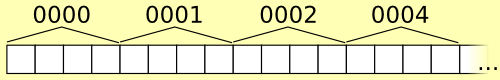
For example, if the fixed-length for sequences is 6 and the stride is 4,000 bytes, looking up “141592” is just a matter of seeking to byte 141,592 * 4,000 and reading in positions until some sort of sentinel. The stride must be long enough to store all the positions for any indexed sequence.

For this purpose, the digits of pi are practically random numbers. The good news is that it means a fixed stride will work well. Any particular sequence appears just as often as any other. The chance a specific n-length sequence begins at a specific position is 1 / 10^n. There are 1 billion positions, so a particular sequence will have 1e9 / 10^n positions associated with it, which is a good place to start for picking a stride.

The bad news is that building the index means jumping around the database essentially at random for each write. This will break any sort of cache between the program and the hard drive. It’s incredibly slow, even mmap()ed. The workaround is to either do it entirely in RAM (needs at least 6GB of RAM for 1 billion digits!) or to build it up over many passes. I didn’t try it on an SSD but maybe the random access is more tolerable there.

Adding an Index

Doing all the work in memory makes it easier to improve the database format anyway. It can be broken into an index section and a tables section. Instead of a fixed stride for the data, front-load the database with a similar index that points to the section (table) of the database file that holds that sequence’s pi positions. Each of the 10^n positions gets a single integer in the index at the front of the file. Looking up the positions for a sequence means parsing the sequence as a number, seeking to that offset into the beginning of the database, reading in another offset integer, and then seeking to that new offset. Now the database is compact and there are no concerns about stride.

No sentinel mark is needed either. The tables are concatenated in order in the table part of the database. To determine where to stop, take a peek at the next sequence’s start offset in the index. Its table immediately follows, so this doubles as an end offset. For convenience, one final integer in the index will point just beyond the end of the database, so the last sequence (99999…) doesn’t require special handling.

Searching Shorter and Longer

If the database built for fixed length sequences, how is a sequence of a different length searched? The two cases, shorter and longer, are handled differently.

If the sequence is shorter, fill in the remaining digits, …000 to …999, and look up each sequence. For example, if n=6 and we’re searching for “1415”, get all the positions for “141500”, “141501”, “141502”, …, “141599” and concatenate them. Fortunately the database already has them stored this way! Look up the offsets for “141500” and “141600” and grab everything in between. The downside is that the pi positions are only partially sorted, so they may require sorting before presenting to the user.

If the sequence is longer, the original digits file will be needed. Get the table for the subsequence fixed-length prefix, then seek into the digits file checking each of the pi positions for a full match. This requires lots of extra seeking, but a long sequence will naturally have fewer positions to test. For example, if n=7 and we’re looking for “141592653”, look up the “1415926” table in the database and check each of its 106 positions.

With this database searches are only a few milliseconds (though very much subject to cache misses). Here’s my program in action, from the repository linked above.

$ time ./pipattern 141592653
1: 14159265358979323
427238911: 14159265303126685
570434346: 14159265337906537
678096434: 14159265360713718

real	0m0.004s
user	0m0.000s
sys	0m0.000s

I call that challenge completed!

A GPU Approach to Voronoi Diagrams

2014-06-01T21:53:48Z

I recently got an itch to play around with Voronoi diagrams. It’s a diagram that divides a space into regions composed of points closest to one of a set of seed points. There are a couple of algorithms for computing a Voronoi diagram: Bowyer-Watson and Fortune. These are complicated and difficult to implement.

However, if we’re interested only in rendering a Voronoi diagram as a bitmap, there’s a trivial brute for algorithm. For every pixel of output, determine the closest seed vertex and color that pixel appropriately. It’s slow, especially as the number of seed vertices goes up, but it works perfectly and it’s dead simple!

Does this strategy seem familiar? It sure sounds a lot like an OpenGL fragment shader! With a shader, I can push the workload off to the GPU, which is intended for this sort of work. Here’s basically what it looks like.

/* voronoi.frag */
uniform vec2 seeds[32];
uniform vec3 colors[32];

void main() {
    float dist = distance(seeds[0], gl_FragCoord.xy);
    vec3 color = colors[0];
    for (int i = 1; i < 32; i++) {
        float current = distance(seeds[i], gl_FragCoord.xy);
        if (current < dist) {
            color = colors[i];
            dist = current;
        }
    }
    gl_FragColor = vec4(color, 1.0);
}

If you have a WebGL-enabled browser, you can see the results for yourself here. Now, as I’ll explain below, what you see here isn’t really this shader, but the result looks identical. There are two different WebGL implementations included, but only the smarter one is active. (There’s also a really slow HTML5 canvas fallback.)

https://skeeto.github.io/voronoi-toy/ (source)

You can click and drag points around the diagram with your mouse. You can add and remove points with left and right clicks. And if you press the “a” key, the seed points will go for a random walk, animating the whole diagram. Here’s a (HTML5) video showing it off.

Unfortunately, there are some serious problems with this approach. It has to do with passing seed information as uniforms.

The number of seed vertices is hardcoded. The shader language requires uniform arrays to have known lengths at compile-time. If I want to increase the number of seed vertices, I need to generate, compile, and link a new shader to replace it. My implementation actually does this. The number is replaced with a %%MAX%% template that I fill in using a regular expression before sending the program off to the GPU.
The number of available uniform bindings is very constrained, even on high-end GPUs: GL_MAX_FRAGMENT_UNIFORM_VECTORS. This value is allowed to be as small as 16! A typical value on high-end graphics cards is a mere 221. Each array element counts as a binding, so our shader may be limited to as few as 8 seed vertices. Even on nice GPUs, we’re absolutely limited to 110 seed vertices. An alternative approach might be passing seed and color information as a texture, but I didn’t try this.
There’s no way to bail out of the loop early, at least with OpenGL ES 2.0 (WebGL) shaders. We can’t break or do any sort of branching on the loop variable. Even if we only have 4 seed vertices, we still have to compare against the full count. The GPU has plenty of time available, so this wouldn’t be a big issue, except that we need to skip over the “unused” seeds somehow. They need to be given unreasonable position values. Infinity would be an unreasonable value (infinitely far away), but GLSL floats aren’t guaranteed to be able to represent infinity. We can’t even know what the maximum floating-point value might be. If we pick something too large, we get an overflow garbage value, such as 0 (!!!) in my experiments.

Because of these limitations, this is not a very good way of going about computing Voronoi diagrams on a GPU. Fortunately there’s a much much better approach!

A Smarter Approach

With the above implemented, I was playing around with the fragment shader, going beyond solid colors. For example, I changed the shade/color based on distance from the seed vertex. A results of this was this “blood cell” image, a difference of a couple lines in the shader.

That’s when it hit me! Render each seed as cone pointed towards the camera in an orthographic projection, coloring each cone according to the seed’s color. The Voronoi diagram would work itself out automatically in the depth buffer. That is, rather than do all this distance comparison in the shader, let OpenGL do its normal job of figuring out the scene geometry.

Here’s a video (GIF) I made that demonstrates what I mean.

Not only is this much faster, it’s also far simpler! Rather than being limited to a hundred or so seed vertices, this version could literally do millions of them, limited only by the available memory for attribute buffers.

The Resolution Catch

There’s a catch, though. There’s no way to perfectly represent a cone in OpenGL. (And if there was, we’d be back at the brute force approach as above anyway.) The cone must be built out of primitive triangles, sort of like pizza slices, using GL_TRIANGLE_FAN mode. Here’s a cone made of 16 triangles.

Unlike the previous brute force approach, this is an approximation of the Voronoi diagram. The more triangles, the better the approximation, converging on the precision of the initial brute force approach. I found that for this project, about 64 triangles was indistinguishable from brute force.

Instancing to the Rescue

At this point things are looking pretty good. On my desktop, I can maintain 60 frames-per-second for up to about 500 seed vertices moving around randomly (“a”). After this, it becomes draw-bound because each seed vertex requires a separate glDrawArrays() call to OpenGL. The workaround for this is an OpenGL extension called instancing. The WebGL extension for instancing is ANGLE_instanced_arrays.

The cone model was already sent to the GPU during initialization, so, without instancing, the draw loop only has to bind the uniforms and call draw for each seed. This code uses my Igloo WebGL library to simplify the API.

var cone = programs.cone.use()
        .attrib('cone', buffers.cone, 3);
for (var i = 0; i < seeds.length; i++) {
    cone.uniform('color', seeds[i].color)
        .uniform('position', seeds[i].position)
        .draw(gl.TRIANGLE_FAN, 66);  // 64 triangles == 66 verts
}

It’s driving this pair of shaders.

/* cone.vert */
attribute vec3 cone;
uniform vec2 position;

void main() {
    gl_Position = vec4(cone.xy + position, cone.z, 1.0);
}

/* cone.frag */
uniform vec3 color;

void main() {
    gl_FragColor = vec4(color, 1.0);
}

Instancing works by adjusting how attributes are stepped. Normally the vertex shader runs once per element, but instead we can ask that some attributes step once per instance, or even once per multiple instances. Uniforms are then converted to vertex attribs and the “loop” runs implicitly on the GPU. The instanced glDrawArrays() call takes one additional argument: the number of instances to draw.

ext = gl.getExtension("ANGLE_instanced_arrays"); // only once

programs.cone.use()
    .attrib('cone', buffers.cone, 3)
    .attrib('position', buffers.positions, 2)
    .attrib('color', buffers.colors, 3);
/* Tell OpenGL these iterate once (1) per instance. */
ext.vertexAttribDivisorANGLE(cone.vars['position'], 1);
ext.vertexAttribDivisorANGLE(cone.vars['color'], 1);
ext.drawArraysInstancedANGLE(gl.TRIANGLE_FAN, 0, 66, seeds.length);

The ugly ANGLE names are because this is an extension, not part of WebGL itself. As such, my program will fall back to use multiple draw calls when the extension is not available. It’s only there for a speed boost.

Here are the new shaders. Notice the uniforms are gone.

/* cone-instanced.vert */
attribute vec3 cone;
attribute vec2 position;
attribute vec3 color;

varying vec3 vcolor;

void main() {
    vcolor = color;
    gl_Position = vec4(cone.xy + position, cone.z, 1.0);
}

/* cone-instanced.frag */
varying vec3 vcolor;

void main() {
    gl_FragColor = vec4(vcolor, 1.0);
}

On the same machine, the instancing version can do a few thousand seed vertices (an order of magnitude more) at 60 frames-per-second, after which it becomes bandwidth saturated. This is because, for the animation, every vertex position is updated on the GPU on each frame. At this point it’s overcrowded anyway, so there’s no need to support more.

Rumor Simulation

2012-03-09T00:00:00Z

A couple months ago someone posted an interesting programming homework problem on reddit, asking for help. Help had already been provided before I got there, but I thought the problem was an interesting one.

Write a program that simulates the spreading of a rumor among a group of people. At any given time, each person in the group is in one of three categories:

IGNORANT - the person has not yet heard the rumor

SPREADER - the person has heard the rumor and is eager to spread it

STIFLER - the person has heard the rumor but considers it old news and will not spread it

At the very beginning, there is one spreader; everyone else is ignorant. Then people begin to encounter each other.

So the encounters go like this:

If a SPREADER and an IGNORANT meet, IGNORANT becomes a SPREADER.

If a SPREADER and a STIFLER meet, the SPREADER becomes a STIFLER.

If a SPREADER and a SPREADER meet, they both become STIFLERS.

In all other encounters nothing changes.

Your program should simulate this by repeatedly selecting two people randomly and having them “meet.”

There are three questions we want to answer:

Will everyone eventually hear the rumor, or will it die out before everyone hears it?

If it does die out, what percentage of the population hears it?

How long does it take? i.e. How many encounters occur before the rumor dies out?

I wrote a very thorough version to produce videos of the simulation in action.

https://github.com/skeeto/rumor-sim

It accepts some command line arguments, so you don’t need to edit any code just to try out some simple things.

And here are a couple of videos. Each individual is a cell in a 2D grid. IGNORANT is black, SPREADER is red, and STIFLER is white. Note that this is not a cellular automata, because cell neighborship does not come into play.

Here’s are the statistics for ten different rumors.

Rumor(n=10000, meetups=132380, knowing=0.789)
Rumor(n=10000, meetups=123944, knowing=0.7911)
Rumor(n=10000, meetups=117459, knowing=0.7985)
Rumor(n=10000, meetups=127063, knowing=0.79)
Rumor(n=10000, meetups=124116, knowing=0.8025)
Rumor(n=10000, meetups=115903, knowing=0.7952)
Rumor(n=10000, meetups=137222, knowing=0.7927)
Rumor(n=10000, meetups=134354, knowing=0.797)
Rumor(n=10000, meetups=113887, knowing=0.8025)
Rumor(n=10000, meetups=139534, knowing=0.7938)

Except for very small populations, the simulation always terminates very close to 80% rumor coverage. I don’t understand (yet) why this is, but I find it very interesting.

Lisp Let in GNU Octave

2012-02-08T00:00:00Z

In BrianScheme, the standard Lisp binding form let isn’t a special form. That is, it’s not a hard-coded language feature, or special form. It’s built on top of lambda. In any lexically-scoped Lisp, the expression,

(let ((x 10)
      (y 20))
  (* 10 20))

Can also be written as,

((lambda (x y)
   (* x y))
 10 20)

BrianScheme’s let is just a macro that transforms into a lambda expression. This is also what made it so important to implement lambda lifting, to optimize these otherwise-expensive forms.

It’s possible to achieve a similar effect in GNU Octave (but not Matlab, due to its flawed parser design). The language permits simple lambda expressions, much like Python.

> f = @(x) x + 10;
> f(4)
ans = 14

It can be used to create a scope in a language that’s mostly devoid of scope. For example, I can avoid assigning a value to a temporary variable just because I need to use it in two places. This one-liner generates a random 3D unit vector.

(@(v) v / norm(v))(randn(1, 3))

The anonymous function is called inside the same expression where it’s created. In practice, doing this is stupid. It’s confusing and there’s really nothing to gain by being clever, doing it in one line instead of two. Most importantly, there’s no macro system that can turn this into a new language feature. However, I enjoyed using this technique to create a one-liner that generates n random unit vectors.

n = 1000;
p = (@(v) v ./ repmat(sqrt(sum(abs(v) .^ 2, 2)), 1, 3))(randn(n, 3));

Why was I doing this? I was using the Monte Carlo method to double-check my solution to this math problem:

What is the average straight line distance between two points on a sphere of radius 1?

I was also demonstrating to Gavin that simply choosing two angles is insufficient, because the points the angles select are not evenly distributed over the surface of the sphere. I generated this video, where the poles are clearly visible due to the uneven selection by two angles.

This took hours to render with gnuplot! Here are stylized versions: Dark and Light.

Cartoon Liquid Simulation

2012-02-03T00:00:00Z

Update June 2013: This program has been ported to WebGL!!!

The other day I came across this neat visual trick: How to simulate liquid (Flash). It’s a really simple way to simulate some natural-looking liquid.

Perform a physics simulation of a number of circular particles.
Render this simulation in high contrast.
Gaussian blur the rendering.
Threshold the blur.

I [made my own version][fun] in Java, using JBox2D for the physics simulation.

https://github.com/skeeto/fun-liquid

For those of you who don’t want to run a Java applet, here’s a video demonstration. Gravity is reversed every few seconds, causing the liquid to slosh up and down over and over. The two triangles on the sides help mix things up a bit. The video flips through the different components of the animation.

It’s not a perfect liquid simulation. The surface never settles down, so the liquid is lumpy, like curdled milk. There’s also a lack of cohesion, since JBox2D doesn’t provide cohesion directly. However, I think I could implement cohesion on my own by writing a custom contact.

JBox2D is a really nice, easy-to-use 2D physics library. I only had to read the first two chapters of the Box2D manual. Everything else can be figured out through the JBox2D Javadocs. It’s also available from the Maven repository, which is the reason I initially selected it. My only complaint so far is that the API doesn’t really follow best practice, but that’s probably because it follows the Box2D C++ API so closely.

I’m excited about JBox2D and I plan on using it again for some future project ideas. Maybe even a game.

The most computationally intensive part of the process isn’t the physics. That’s really quite cheap. It’s actually blurring, by far. Blurring involves convolving a kernel over the image — O(n^2) time. The graphics card would be ideal for that step, probably eliminating it as a bottleneck, but it’s unavailable to pure Java. I could have pulled in lwjgl, but I wanted to keep it simple, so that it could be turned into a safe applet.

As a result, it may not run smoothly on computers that are more than a couple of years old. I’ve been trying to come up with a cheaper alternative, such as rendering a transparent halo around each ball, but haven’t found anything yet. Even with that fix, thresholding would probably be the next bottleneck — something else the graphics card would be really good at.

Silky Smooth Perlin Noise Surface

2012-01-19T00:00:00Z

At work I’ve recently been generating viewsheds over DTED sets. Earlier this week I was asked to give an informal presentation on what I was doing. I wanted some terrain that demonstrated some key features, such as vision being occluded by hills of varying heights. Rather than search through the available DTED files for something good, I opted for generating my own terrain, using an old trick of mine: my noise “cloud” generator. That’s a lesson in the usefulness of maintaining a blog. The useful things you learn and create are easy to revisit years later!

I generated some noise, looked at it with surf(), and repeated until I found something useful. (Update June 2012: the function is called perlin() but it’s not actually Perlin noise.)

m = perlin(1024);
surf(m);

The generated terrain is really quite rough, so I decided to smooth it out by convolving it with a 2-dimensional Gaussian kernel.

k = fspecial('gaussian', 9);
ms = conv2(m, k, 'same');

It still wasn’t smooth enough. So I repeated the process a bit,

for i = 1:10
    ms = conv2(ms, k, 'same');
end

Perfect! I used that for my presentation. However, I was having fun and decided to experiment more with this. I filtered it again another 1000 times and generated a surf() plot with a high-resolution colormap — the default colormap size caused banding.

colormap(copper(1024));
surf(ms, 'EdgeAlpha', 0);
axis('equal');

It produced this beautiful result!

I think it looks like a photograph from a high-powered microscope, or maybe the turbulent surface of some kind of creamy beverage being stirred.

At work when I need something Matlab-ish, I use Octave about half the time and Matlab the other half. In this case, I was using Matlab. Octave doesn’t support the EdgeAlpha property, nor the viewshed() function that I needed for my work. Matlab currently makes much prettier plots than Octave.

Unorderable Sets

2009-09-27T00:00:00Z

Under Gavin's suggestion, I've been watching The Prisoner, a 1960's British television show. The main character is an ex-spy held prisoner in "the Village", an Orwellian, isolated, enclosed town. No one in the Village has a name, but is instead assigned a number. The main character's number is 6.

As far as I can tell, after number 2 the order of the numbers is not important. Number 56 is no more important than number 12. By using numbers to name things there is an implied ordering, even if the the ordering is insignificant. It could be misleading to a newcomer.

Is there an unordered set could be used to name things? More specifically, is there a set that cannot be ordered? If it is unorderable then there is no implicit ordering to cause confusion. It's easy to have an unorderable set in theory, but I think it is difficult to have in practice.

Using letters is obviously out, as the alphabet has an order. Words and names made of letters can be sorted according to the alphabet. However, the ability to order words is almost never used outside of indexing. If words are used to name things, a newcomer is unlikely to assume relationships based on ordering. No one will assume Alan is more important than Bob.

Large numbers also tend to lack an assumed order. I don't think anyone assumes a larger or smaller social security number has meaning, or a larger or smaller phone number. However, these values are also known to be handed out in some semi-random way.

But can we do better? For at least English speakers, is it possible to create an unorderable set? If the items in the set have a vocal pronunciation, then they can probably be ordered by their phonetics. That could be avoided by using non-standard phonetic components, like clicks and pops, which won't have a standard ordering (in English, anyway).

A set has an order if there is a total, transitive, relational operator for the set. If such an operator does not exist then the set isn't linearly ordered. I want a set that can't easily have such an operator.

If a set of symbols was created, how might they be presented as to show no ordering. The order of the symbols in the original presentation might be considered the ordering, like how the alphabet is always presented in order. A circle could be used, but this is circularly ordered. I think there is also the issue of memorization. A human will have a much better time memorizing the symbols if memorized in some order. For example, try naming all the letters of the alphabet at random, without repeats. Or US states.

Thanks to modern day technology, with dynamic content, the set could be displayed in a random order each time it is viewed. For a web page, the server could select a random order, or a JavaScript program could reorder the images at random.

There could be partially ordered sets, like hierarchies and DAGs. The ordering in The Prisoner is one of these. There is number 1, then number 2, then everyone else. Is there a partially ordered set in use that has unique names at the same level?

The penalties incurred by intentionally prohibiting order would likely outweigh the benefit of the set. If it's not orderable, we can't index it, and it's difficult to deal with. I expect it's much easer to just use numbers and tell people that the order isn't important, or just use an obviously unordered set.

United States Hamiltonian Paths

2009-06-21T00:00:00Z

Awhile ago I wanted to find every Hamiltonian path in the contiguous 48 states. That is, trips that visit each state exactly once. Writing a program to search for Hamiltonian paths is easy (I did this already). The most time consuming part was actually putting together the data that specified the graph to be searched. I hope someone somewhere finds it useful. Here is a map for reference,

It took me several passes before I stopped finding errors. I think I have it all right now, but there could still be some mistakes. If you see one, leave a comment and I'll fix it here. Here is the graph as an S-expression alist; the car (first) element in each list is a state, and the cdr (rest) is the unordered list of states that can be reached from it.

((me nh)
 (nh vt ma me)
 (vt ny ma nh)
 (ma ri ct ny nh vt)
 (ny pa nj ma ct vt)
 (ri ma ct)
 (ct ri ma ny)
 (nj pa ny de)
 (de md pa nj)
 (pa nj ny de md wv oh)
 (md pa de va wv)
 (va md wv ky tn nc)
 (nc va tn ga sc)
 (sc nc ga)
 (ga fl sc al nc tn)
 (al ms fl ga tn)
 (ms la ar tn al)
 (tn ms al ga nc va ky mo ar)
 (ky wv va tn mo il in oh)
 (wv md pa oh ky va)
 (oh pa wv ky in mi)
 (fl al ga)
 (mi wi oh in)
 (wi mn ia il mi)
 (il in ky mo ia wi)
 (in oh ky il mi)
 (mo il ky tn ar ok ks ne ia)
 (ar mo tn ms la tx ok)
 (la ms ar tx)
 (tx ok nm ar la)
 (ok ks mo ar tx nm co)
 (ks ok co ne mo)
 (ne sd ia mo ks co wy)
 (sd nd mn ia ne wy mt)
 (nd mt sd mn)
 (ia ne mo il wi mn sd)
 (mn wi ia sd nd)
 (mt id wy sd nd)
 (wy id ut co ne sd mt)
 (co ne ks ok nm ut wy)
 (nm co ok tx az)
 (az nm ut ca nv)
 (ut nv id wy co az)
 (id mt wy ut nv or wa)
 (wa or id)
 (or wa id nv ca)
 (nv or id ut az ca)
 (ca az nv or))

Note that all paths must start or end in Maine because it connects to only one other state.

Brainfuck Halting Problem

2009-04-12T00:00:00Z

On my brainfuck compiler project, I proposed pre-calculation as an optimization technique. The idea can work, but it has an issue that will always be unsolvable: how do you know that the pre-calculation will halt? This is called the halting problem and it has been proven impossible to solve.

The idea was that the compiler would run the brainfuck program up until the first input operation — if there even was one. It would record all output and the final state of the memory. Instead of compiling the code was was run, it would compile code that would print all of the output and set the memory at the final state.

I has mistakenly assumed that it would be possible to detect a non-halting program and avoid doing pre-calculation on it. I described how it would be done and left it at that. Recently, someone kindly sent me an email containing only 5 letters:

+[--]

This defeated my ill-conceived idea.

Because brainfuck is Turing complete, it is actually impossible to determine whether or not an arbitrary brainfuck loop will halt. A computer can't do it. A human brain (a fancy computer) can't do it either. It cannot be done, at least not in this universe.

So, if implemented, this pre-calculation measure will always be flawed.