Articles tagged media at null program

You might not need machine learning

2020-11-24T04:04:36Z

This article was discussed on Hacker News.

Machine learning is a trendy topic, so naturally it’s often used for inappropriate purposes where a simpler, more efficient, and more reliable solution suffices. The other day I saw an illustrative and fun example of this: Neural Network Cars and Genetic Algorithms. The video demonstrates 2D cars driven by a neural network with weights determined by a generic algorithm. However, the entire scheme can be replaced by a first-degree polynomial without any loss in capability. The machine learning part is overkill.

Above demonstrates my implementation using a polynomial to drive the cars. My wife drew the background. There’s no path-finding; these cars are just feeling their way along the track, “following the rails” so to speak.

My intention is not to pick on this project in particular. The likely motivation in the first place was a desire to apply a neural network to something. Many of my own projects are little more than a vehicle to try something new, so I can sympathize. Though a professional setting is different, where machine learning should be viewed with a more skeptical eye than it’s usually given. For instance, don’t use active learning to select sample distribution when a quasirandom sequence will do.

In the video, the car has a limited turn radius, and minimum and maximum speeds. (I’ve retained these contraints in my own simulation.) There are five sensors — forward, forward-diagonals, and sides — each sensing the distance to the nearest wall. These are fed into a 3-layer neural network, and the outputs determine throttle and steering. Sounds pretty cool!

A key feature of neural networks is that the outputs are a nonlinear function of the inputs. However, steering a 2D car is simple enough that a linear function is more than sufficient, and neural networks are unnecessary. Here are my equations:

steering = C0*input1 - C0*input3
throttle = C1*input2

I only need three of the original inputs — forward for throttle, and diagonals for steering — and the driver has just two parameters, C0 and C1, the polynomial coefficients. Optimal values depend on the track layout and car configuration, but for my simulation, most values above 0 and below 1 are good enough in most cases. It’s less a matter of crashing and more about navigating the course quickly.

The lengths of the red lines below are the driver’s three inputs:

These polynomials are obviously much faster than a neural network, but they’re also easy to understand and debug. I can confidently reason about the entire range of possible inputs rather than worry about a trained neural network responding strangely to untested inputs.

Instead of doing anything fancy, my program generates the coefficients at random to explore the space. If I wanted to generate a good driver for a course, I’d run a few thousand of these and pick the coefficients that complete the course in the shortest time. For instance, these coefficients make for a fast, capable driver for the course featured at the top of the article:

C0 = 0.896336973, C1 = 0.0354805067

Many constants can complete the track, but some will be faster than others. If I was developing a racing game using this as the AI, I’d not just pick constants that successfully complete the track, but the ones that do it quickly. Here’s what the spread can look like:

If you want to play around with this yourself, here’s my C source code that implements this driving AI and generates the videos and images above:

aidrivers.c

Racetracks are just images drawn in your favorite image editing program using the colors documented in the source header.

Netpbm Animation Showcase

2020-06-29T21:03:02Z

Ever since I worked out how to render video from scratch some years ago, it’s been an indispensable tool in my software development toolbelt. It’s the first place I reach when I need to display some graphics, even if it means having to do the rendering myself. I’ve used it often in throwaway projects in a disposable sort of way. More recently, though, I’ve kept better track of these animations since some of them are pretty cool, and I’d like to look a them again. This post is a showcase of some of these projects.

Each project is in a ready-to-run state of compile, then run with the output piped into a media player or video encoding. The header includes the exactly commands you need. Since that’s probably inconvenient for most readers, I’ve included a pre-recorded sample of each. Though in a few cases, especially those displaying random data, video encoding really takes something away from the final result, and it may be worth running yourself.

The projects are not in any particular order.

RANDU

Source: randu.c

This is a little demonstration of the poor quality of the RANDU pseudorandom number generator. Note how the source embeds a monospace font so that it can render the text in the corner. For the 3D effect, it includes an orthographic projection function. This function will appear again later since I tend to cannibalize my own projects.

Color sorting

Source: colorsort.c

The original idea came from an old reddit post.

Kruskal maze generator

Source: animaze.c

This effect was invented by my current mentee student while working on maze / dungeon generation late last year. This particular animation is my own implementation. It outputs Netpbm by default, but, for both fun and practice, also includes an entire implementation in OpenGL. It’s enabled at compile time with -DENABLE_GL so long as you have GLFW and GLEW (even on Windows!).

Sliding rooks puzzle

Source: rooks.c

I wanted to watch an animated solution to the sliding rooks puzzle. This program solves the puzzle using a bitboard, then animates the solution. The rook images are embedded in the program, compressed using a custom run-length encoding (RLE) scheme with a tiny palette.

Glauber’s dynamics

Source: magnet.c

My own animation of Glauber’s dynamics using a totally unoriginal color palette.

Fire

Source: fire.c

This is the classic Doom fire animation. I later implemented it in WebGL with a modified algorithm.

Mersenne Twister

Source: mtvisualize.c

A visualization of the Mersenne Twister pseudorandom number generator. Not terribly interesting, so I almost didn’t include it.

Pixel sorting

Source: pixelsort.c

Another animation inspired by a reddit post. Starting from the top-left corner, swap the current pixel to the one most like its neighbors.

Random walk (2D)

Source: walkers.c

Another reproduction of a reddit post. This is recent enough that I’m using a disposable LCG.

Manhattan distance Voronoi diagram

Source: voronoi.c

Another reddit post, though I think my version looks a lot nicer. I like to play this one over and over on repeat with different seeds.

Random walk (3D)

Source: walk3d.c

Another ~~stolen idea~~ personal take on a reddit post. This features the orthographic projection function from the RANDU animation. Video encoding makes a real mess of this one, and I couldn’t work out encoding options to make it look nice, so this one looks a lot better “in person.”

Lorenz system

Source: lorenz.c

A 3D animation I adapted from the 3D random walk above, meaning it uses the same orthographic projection. I have a WebGL version of this one, but I like that I could do this in such a small amount of code and without an existing rendering engine. Like before, this is really damaged by video encoding and is best seen live.

Bonus: I made an obfuscated version just to show how small this can get!

When Parallel: Pull, Don't Push

2020-04-30T22:35:51Z

This article was discussed on Hacker News.

I’ve noticed a small pattern across a few of my projects where I had vectorized and parallelized some code. The original algorithm had a “push” approach, the optimized version instead took a “pull” approach. In this article I’ll describe what I mean, though it’s mostly just so I can show off some pretty videos, pictures, and demos.

Sandpiles

A good place to start is the Abelian sandpile model, which, like many before me, completely captured my attention for awhile. It’s a cellular automaton where each cell is a pile of grains of sand — a sandpile. At each step, any sandpile with more than four grains of sand spill one grain into its four 4-connected neighbors, regardless of the number of grains in those neighboring cell. Cells at the edge spill their grains into oblivion, and those grains no longer exist.

With excess sand falling over the edge, the model eventually hits a stable state where all piles have three or fewer grains. However, until it reaches stability, all sorts of interesting patterns ripple though the cellular automaton. In certain cases, the final pattern itself is beautiful and interesting.

Numberphile has a great video describing how to form a group over recurrent configurations (also). In short, for any given grid size, there’s a stable identity configuration that, when “added” to any other element in the group will stabilize back to that element. The identity configuration is a fractal itself, and has been a focus of study on its own.

Computing the identity configuration is really just about running the simulation to completion a couple times from certain starting configurations. Here’s an animation of the process for computing the 64x64 identity configuration:

As a fractal, the larger the grid, the more self-similar patterns there are to observe. There are lots of samples online, and the biggest I could find was this 3000x3000 on Wikimedia Commons. But I wanted to see one that’s even bigger, damnit! So, skipping to the end, I eventually computed this 10000x10000 identity configuration:

This took 10 days to compute using my optimized implementation:

https://github.com/skeeto/scratch/blob/master/animation/sandpiles.c

I picked an algorithm described in a code golf challenge:

f(ones(n)*6 - f(ones(n)*6))

Where f() is the function that runs the simulation to a stable state.

I used OpenMP to parallelize across cores, and SIMD to parallelize within a thread. Each thread operates on 32 sandpiles at a time. To compute the identity sandpile, each sandpile only needs 3 bits of state, so this could potentially be increased to 85 sandpiles at a time on the same hardware. The output format is my old mainstay, Netpbm, including the video output.

Sandpile push and pull

So, what do I mean about pushing and pulling? The naive approach to simulating sandpiles looks like this:

for each i in sandpiles {
    if input[i] < 4 {
        output[i] = input[i]
    } else {
        output[i] = input[i] - 4
        for each j in neighbors {
            output[j] = output[j] + 1
        }
    }
}

As the algorithm examines each cell, it pushes results into neighboring cells. If we’re using concurrency, that means multiple threads of execution may be mutating the same cell, which requires synchronization — locks, atomics, etc. That much synchronization is the death knell of performance. The threads will spend all their time contending for the same resources, even if it’s just false sharing.

The solution is to pull grains from neighbors:

for each i in sandpiles {
    if input[i] < 4 {
        output[i] = input[i]
    } else {
        output[i] = input[i] - 4
    }
    for each j in neighbors {
        if input[j] >= 4 {
            output[i] = output[i] + 1
        }
    }
}

Each thread only modifies one cell — the cell it’s in charge of updating — so no synchronization is necessary. It’s shader-friendly and should sound familiar if you’ve seen my WebGL implementation of Conway’s Game of Life. It’s essentially the same algorithm. If you chase down the various Abelian sandpile references online, you’ll eventually come across a 2017 paper by Cameron Fish about running sandpile simulations on GPUs. He cites my WebGL Game of Life article, bringing everything full circle. We had spoken by email at the time, and he shared his interactive simulation with me.

Vectorizing this algorithm is straightforward: Load multiple piles at once, one per SIMD channel, and use masks to implement the branches. In my code I’ve also unrolled the loop. To avoid bounds checking in the SIMD code, I pad the state data structure with zeros so that the edge cells have static neighbors and are no longer special.

WebGL Fire

Back in the old days, one of the cool graphics tricks was fire animations. It was so easy to implement on limited hardware. In fact, the most obvious way to compute it was directly in the framebuffer, such as in the VGA buffer, with no outside state.

There’s a heat source at the bottom of the screen, and the algorithm runs from bottom up, propagating that heat upwards randomly. Here’s the algorithm using traditional screen coordinates (top-left corner origin):

func rand(min, max) // random integer in [min, max]

for each x, y from bottom {
    buf[y-1][x+rand(-1, 1)] = buf[y][x] - rand(0, 1)
}

As a push algorithm it works fine with a single-thread, but it doesn’t translate well to modern video hardware. So convert it to a pull algorithm!

for each x, y {
    sx = x + rand(-1, 1)
    sy = y + rand(1, 2)
    output[y][x] = input[sy][sx] - rand(0, 1)
}

Cells pull the fire upward from the bottom. Though this time there’s a catch: This algorithm will have subtly different results.

In the original, there’s a single state buffer and so a flame could propagate upwards multiple times in a single pass. I’ve compensated here by allowing a flames to propagate further at once.
In the original, a flame only propagates to one other cell. In this version, two cells might pull from the same flame, cloning it.

In the end it’s hard to tell the difference, so this works out.

source code and instructions

There’s still potentially contention in that rand() function, but this can be resolved with a hash function that takes x and y as inputs.

Render Multimedia in Pure C

2017-11-03T22:31:15Z

Update 2020: I’ve produced many more examples over the years (even more).

In a previous article I demonstrated video filtering with C and a unix pipeline. Thanks to the ubiquitous support for the ridiculously simple Netpbm formats — specifically the “Portable PixMap” (.ppm, P6) binary format — it’s trivial to parse and produce image data in any language without image libraries. Video decoders and encoders at the ends of the pipeline do the heavy lifting of processing the complicated video formats actually used to store and transmit video.

Naturally this same technique can be used to produce new video in a simple program. All that’s needed are a few functions to render artifacts — lines, shapes, etc. — to an RGB buffer. With a bit of basic sound synthesis, the same concept can be applied to create audio in a separate audio stream — in this case using the simple (but not as simple as Netpbm) WAV format. Put them together and a small, standalone program can create multimedia.

Here’s the demonstration video I’ll be going through in this article. It animates and visualizes various in-place sorting algorithms (see also). The elements are rendered as colored dots, ordered by hue, with red at 12 o’clock. A dot’s distance from the center is proportional to its corresponding element’s distance from its correct position. Each dot emits a sinusoidal tone with a unique frequency when it swaps places in a particular frame.

Original credit for this visualization concept goes to w0rthy.

All of the source code (less than 600 lines of C), ready to run, can be found here:

https://github.com/skeeto/sort-circle

On any modern computer, rendering is real-time, even at 60 FPS, so you may be able to pipe the program’s output directly into your media player of choice. (If not, consider getting a better media player!)

$ ./sort | mpv --no-correct-pts --fps=60 -

VLC requires some help from ppmtoy4m:

$ ./sort | ppmtoy4m -F60:1 | vlc -

Or you can just encode it to another format. Recent versions of libavformat can input PPM images directly, which means x264 can read the program’s output directly:

$ ./sort | x264 --fps 60 -o video.mp4 /dev/stdin

By default there is no audio output. I wish there was a nice way to embed audio with the video stream, but this requires a container and that would destroy all the simplicity of this project. So instead, the -a option captures the audio in a separate file. Use ffmpeg to combine the audio and video into a single media file:

$ ./sort -a audio.wav | x264 --fps 60 -o video.mp4 /dev/stdin
$ ffmpeg -i video.mp4 -i audio.wav -vcodec copy -acodec mp3 \
         combined.mp4

You might think you’ll be clever by using mkfifo (i.e. a named pipe) to pipe both audio and video into ffmpeg at the same time. This will only result in a deadlock since neither program is prepared for this. One will be blocked writing one stream while the other is blocked reading on the other stream.

Several years ago my intern and I used the exact same pure C rendering technique to produce these raytracer videos:

I also used this technique to illustrate gap buffers.

Pixel format and rendering

This program really only has one purpose: rendering a sorting video with a fixed, square resolution. So rather than write generic image rendering functions, some assumptions will be hard coded. For example, the video size will just be hard coded and assumed square, making it simpler and faster. I chose 800x800 as the default:

#define S     800

Rather than define some sort of color struct with red, green, and blue fields, color will be represented by a 24-bit integer (long). I arbitrarily chose red to be the most significant 8 bits. This has nothing to do with the order of the individual channels in Netpbm since these integers are never dumped out. (This would have stupid byte-order issues anyway.) “Color literals” are particularly convenient and familiar in this format. For example, the constant for pink: 0xff7f7fUL.

In practice the color channels will be operated upon separately, so here are a couple of helper functions to convert the channels between this format and normalized floats (0.0–1.0).

static void
rgb_split(unsigned long c, float *r, float *g, float *b)
{
    *r = ((c >> 16) / 255.0f);
    *g = (((c >> 8) & 0xff) / 255.0f);
    *b = ((c & 0xff) / 255.0f);
}

static unsigned long
rgb_join(float r, float g, float b)
{
    unsigned long ir = roundf(r * 255.0f);
    unsigned long ig = roundf(g * 255.0f);
    unsigned long ib = roundf(b * 255.0f);
    return (ir << 16) | (ig << 8) | ib;
}

Originally I decided the integer form would be sRGB, and these functions handled the conversion to and from sRGB. Since it had no noticeable effect on the output video, I discarded it. In more sophisticated rendering you may want to take this into account.

The RGB buffer where images are rendered is just a plain old byte buffer with the same pixel format as PPM. The ppm_set() function writes a color to a particular pixel in the buffer, assumed to be S by S pixels. The complement to this function is ppm_get(), which will be needed for blending.

static void
ppm_set(unsigned char *buf, int x, int y, unsigned long color)
{
    buf[y * S * 3 + x * 3 + 0] = color >> 16;
    buf[y * S * 3 + x * 3 + 1] = color >>  8;
    buf[y * S * 3 + x * 3 + 2] = color >>  0;
}

static unsigned long
ppm_get(unsigned char *buf, int x, int y)
{
    unsigned long r = buf[y * S * 3 + x * 3 + 0];
    unsigned long g = buf[y * S * 3 + x * 3 + 1];
    unsigned long b = buf[y * S * 3 + x * 3 + 2];
    return (r << 16) | (g << 8) | b;
}

Since the buffer is already in the right format, writing an image is dead simple. I like to flush after each frame so that observers generally see clean, complete frames. It helps in debugging.

static void
ppm_write(const unsigned char *buf, FILE *f)
{
    fprintf(f, "P6\n%d %d\n255\n", S, S);
    fwrite(buf, S * 3, S, f);
    fflush(f);
}

Dot rendering

If you zoom into one of those dots, you may notice it has a nice smooth edge. Here’s one rendered at 30x the normal resolution. I did not render, then scale this image in another piece of software. This is straight out of the C program.

In an early version of this program I used a dumb dot rendering routine. It took a color and a hard, integer pixel coordinate. All the pixels within a certain distance of this coordinate were set to the color, everything else was left alone. This had two bad effects:

Dots jittered as they moved around since their positions were rounded to the nearest pixel for rendering. A dot would be centered on one pixel, then suddenly centered on another pixel. This looked bad even when those pixels were adjacent.
There’s no blending between dots when they overlap, making the lack of anti-aliasing even more pronounced.

Instead the dot’s position is computed in floating point and is actually rendered as if it were between pixels. This is done with a shader-like routine that uses smoothstep — just as found in shader languages — to give the dot a smooth edge. That edge is blended into the image, whether that’s the background or a previously-rendered dot. The input to the smoothstep is the distance from the floating point coordinate to the center (or corner?) of the pixel being rendered, maintaining that between-pixel smoothness.

Rather than dump the whole function here, let’s look at it piece by piece. I have two new constants to define the inner dot radius and the outer dot radius. It’s smooth between these radii.

#define R0    (S / 400.0f)  // dot inner radius
#define R1    (S / 200.0f)  // dot outer radius

The dot-drawing function takes the image buffer, the dot’s coordinates, and its foreground color.

static void
ppm_dot(unsigned char *buf, float x, float y, unsigned long fgc);

The first thing to do is extract the color components.

    float fr, fg, fb;
    rgb_split(fgc, &fr, &fg, &fb);

Next determine the range of pixels over which the dot will be draw. These are based on the two radii and will be used for looping.

    int miny = floorf(y - R1 - 1);
    int maxy = ceilf(y + R1 + 1);
    int minx = floorf(x - R1 - 1);
    int maxx = ceilf(x + R1 + 1);

Here’s the loop structure. Everything else will be inside the innermost loop. The dx and dy are the floating point distances from the center of the dot.

    for (int py = miny; py <= maxy; py++) {
        float dy = py - y;
        for (int px = minx; px <= maxx; px++) {
            float dx = px - x;
            /* ... */
        }
    }

Use the x and y distances to compute the distance and smoothstep value, which will be the alpha. Within the inner radius the color is on 100%. Outside the outer radius it’s 0%. Elsewhere it’s something in between.

            float d = sqrtf(dy * dy + dx * dx);
            float a = smoothstep(R1, R0, d);

Get the background color, extract its components, and blend the foreground and background according to the computed alpha value. Finally write the pixel back into the buffer.

            unsigned long bgc = ppm_get(buf, px, py);
            float br, bg, bb;
            rgb_split(bgc, &br, &bg, &bb);

            float r = a * fr + (1 - a) * br;
            float g = a * fg + (1 - a) * bg;
            float b = a * fb + (1 - a) * bb;
            ppm_set(buf, px, py, rgb_join(r, g, b));

That’s all it takes to render a smooth dot anywhere in the image.

Rendering the array

The array being sorted is just a global variable. This simplifies some of the sorting functions since a few are implemented recursively. They can call for a frame to be rendered without needing to pass the full array. With the dot-drawing routine done, rendering a frame is easy:

#define N     360           // number of dots

static int array[N];

static void
frame(void)
{
    static unsigned char buf[S * S * 3];
    memset(buf, 0, sizeof(buf));
    for (int i = 0; i < N; i++) {
        float delta = abs(i - array[i]) / (N / 2.0f);
        float x = -sinf(i * 2.0f * PI / N);
        float y = -cosf(i * 2.0f * PI / N);
        float r = S * 15.0f / 32.0f * (1.0f - delta);
        float px = r * x + S / 2.0f;
        float py = r * y + S / 2.0f;
        ppm_dot(buf, px, py, hue(array[i]));
    }
    ppm_write(buf, stdout);
}

The buffer is static since it will be rather large, especially if S is cranked up. Otherwise it’s likely to overflow the stack. The memset() fills it with black. If you wanted a different background color, here’s where you change it.

For each element, compute its delta from the proper array position, which becomes its distance from the center of the image. The angle is based on its actual position. The hue() function (not shown in this article) returns the color for the given element.

With the frame() function complete, all I need is a sorting function that calls frame() at appropriate times. Here are a couple of examples:

static void
shuffle(int array[N], uint64_t *rng)
{
    for (int i = N - 1; i > 0; i--) {
        uint32_t r = pcg32(rng) % (i + 1);
        swap(array, i, r);
        frame();
    }
}

static void
sort_bubble(int array[N])
{
    int c;
    do {
        c = 0;
        for (int i = 1; i < N; i++) {
            if (array[i - 1] > array[i]) {
                swap(array, i - 1, i);
                c = 1;
            }
        }
        frame();
    } while (c);
}

Synthesizing audio

To add audio I need to keep track of which elements were swapped in this frame. When producing a frame I need to generate and mix tones for each element that was swapped.

Notice the swap() function above? That’s not just for convenience. That’s also how things are tracked for the audio.

static int swaps[N];

static void
swap(int a[N], int i, int j)
{
    int tmp = a[i];
    a[i] = a[j];
    a[j] = tmp;
    swaps[(a - array) + i]++;
    swaps[(a - array) + j]++;
}

Before we get ahead of ourselves I need to write a WAV header. Without getting into the purpose of each field, just note that the header has 13 fields, followed immediately by 16-bit little endian PCM samples. There will be only one channel (monotone).

#define HZ    44100         // audio sample rate

static void
wav_init(FILE *f)
{
    emit_u32be(0x52494646UL, f); // "RIFF"
    emit_u32le(0xffffffffUL, f); // file length
    emit_u32be(0x57415645UL, f); // "WAVE"
    emit_u32be(0x666d7420UL, f); // "fmt "
    emit_u32le(16,           f); // struct size
    emit_u16le(1,            f); // PCM
    emit_u16le(1,            f); // mono
    emit_u32le(HZ,           f); // sample rate (i.e. 44.1 kHz)
    emit_u32le(HZ * 2,       f); // byte rate
    emit_u16le(2,            f); // block size
    emit_u16le(16,           f); // bits per sample
    emit_u32be(0x64617461UL, f); // "data"
    emit_u32le(0xffffffffUL, f); // byte length
}

Rather than tackle the annoying problem of figuring out the total length of the audio ahead of time, I just wave my hands and write the maximum possible number of bytes (0xffffffff). Most software that can read WAV files will understand this to mean the entire rest of the file contains samples.

With the header out of the way all I have to do is write 1/60th of a second worth of samples to this file each time a frame is produced. That’s 735 samples (1,470 bytes) at 44.1kHz.

The simplest place to do audio synthesis is in frame() right after rendering the image.

#define FPS   60            // output framerate
#define MINHZ 20            // lowest tone
#define MAXHZ 1000          // highest tone

static void
frame(void)
{
    /* ... rendering ... */

    /* ... synthesis ... */
}

With the largest tone frequency at 1kHz, Nyquist says we only need to sample at 2kHz. 8kHz is a very common sample rate and gives some overhead space, making it a good choice. However, I found that audio encoding software was a lot happier to accept the standard CD sample rate of 44.1kHz, so I stuck with that.

The first thing to do is to allocate and zero a buffer for this frame’s samples.

    int nsamples = HZ / FPS;
    static float samples[HZ / FPS];
    memset(samples, 0, sizeof(samples));

Next determine how many “voices” there are in this frame. This is used to mix the samples by averaging them. If an element was swapped more than once this frame, it’s a little louder than the others — i.e. it’s played twice at the same time, in phase.

    int voices = 0;
    for (int i = 0; i < N; i++)
        voices += swaps[i];

Here’s the most complicated part. I use sinf() to produce the sinusoidal wave based on the element’s frequency. I also use a parabola as an envelope to shape the beginning and ending of this tone so that it fades in and fades out. Otherwise you get the nasty, high-frequency “pop” sound as the wave is given a hard cut off.

    for (int i = 0; i < N; i++) {
        if (swaps[i]) {
            float hz = i * (MAXHZ - MINHZ) / (float)N + MINHZ;
            for (int j = 0; j < nsamples; j++) {
                float u = 1.0f - j / (float)(nsamples - 1);
                float parabola = 1.0f - (u * 2 - 1) * (u * 2 - 1);
                float envelope = parabola * parabola * parabola;
                float v = sinf(j * 2.0f * PI / HZ * hz) * envelope;
                samples[j] += swaps[i] * v / voices;
            }
        }
    }

Finally I write out each sample as a signed 16-bit value. I flush the frame audio just like I flushed the frame image, keeping them somewhat in sync from an outsider’s perspective.

    for (int i = 0; i < nsamples; i++) {
        int s = samples[i] * 0x7fff;
        emit_u16le(s, wav);
    }
    fflush(wav);

Before returning, reset the swap counter for the next frame.

    memset(swaps, 0, sizeof(swaps));

Font rendering

You may have noticed there was text rendered in the corner of the video announcing the sort function. There’s font bitmap data in font.h which gets sampled to render that text. It’s not terribly complicated, but you’ll have to study the code on your own to see how that works.

Learning more

This simple video rendering technique has served me well for some years now. All it takes is a bit of knowledge about rendering. I learned quite a bit just from watching Handmade Hero, where Casey writes a software renderer from scratch, then implements a nearly identical renderer with OpenGL. The more I learn about rendering, the better this technique works.

Before writing this post I spent some time experimenting with using a media player as a interface to a game. For example, rather than render the game using OpenGL or similar, render it as PPM frames and send it to the media player to be displayed, just as game consoles drive television sets. Unfortunately the latency is horrible — multiple seconds — so that idea just doesn’t work. So while this technique is fast enough for real time rendering, it’s no good for interaction.

Rolling Shutter Simulation in C

2017-07-02T18:35:16Z

The most recent Smarter Every Day (#172) explains a phenomenon that results from rolling shutter. You’ve likely seen this effect in some of your own digital photographs. When a CMOS digital camera captures a picture, it reads one row of the sensor at a time. If the subject of the picture is a fast-moving object (relative to the camera), then the subject will change significantly while the image is being captured, giving strange, unreal results:

In the Smarter Every Day video, Destin illustrates the effect by simulating rolling shutter using a short video clip. In each frame of the video, a few additional rows are locked in place, showing the effect in slow motion, making it easier to understand.

At the end of the video he thanks a friend for figuring out how to get After Effects to simulate rolling shutter. After thinking about this for a moment, I figured I could easily accomplish this myself with just a bit of C, without any libraries. The video above this paragraph is the result.

I previously described a technique to edit and manipulate video without any formal video editing tools. A unix pipeline is sufficient for doing minor video editing, especially without sound. The program at the front of the pipe decodes the video into a raw, uncompressed format, such as YUV4MPEG or PPM. The tools in the middle losslessly manipulate this data to achieve the desired effect (watermark, scaling, etc.). Finally, the tool at the end encodes the video into a standard format.

$ decode video.mp4 | xform-a | xform-b | encode out.mp4

For the “decode” program I’ll be using ffmpeg now that it’s back in the Debian repositories. You can throw a video in virtually any format at it and it will write PPM frames to standard output. For the encoder I’ll be using the x264 command line program, though ffmpeg could handle this part as well. Without any filters in the middle, this example will just re-encode a video:

$ ffmpeg -i input.mp4 -f image2pipe -vcodec ppm pipe:1 | \
    x264 -o output.mp4 /dev/stdin

The filter tools in the middle only need to read and write in the raw image format. They’re a little bit like shaders, and they’re easy to write. In this case, I’ll write C program that simulates rolling shutter. The filter could be written in any language that can read and write binary data from standard input to standard output.

Update: It appears that input PPM streams are a rather recent feature of libavformat (a.k.a lavf, used by x264). Support for PPM input first appeared in libavformat 3.1 (released June 26th, 2016). If you’re using an older version of libavformat, you’ll need to stick ppmtoy4m in front of x264 in the processing pipeline.

$ ffmpeg -i input.mp4 -f image2pipe -vcodec ppm pipe:1 | \
    ppmtoy4m | \
    x264 -o output.mp4 /dev/stdin

Video filtering in C

In the past, my go to for raw video data has been loose PPM frames and YUV4MPEG streams (via ppmtoy4m). Fortunately, over the years a lot of tools have gained the ability to manipulate streams of PPM images, which is a much more convenient format. Despite being raw video data, YUV4MPEG is still a fairly complex format with lots of options and annoying colorspace concerns. PPM is simple RGB without complications. The header is just text:

P6

The maximum depth is virtually always 255. A smaller value reduces the image’s dynamic range without reducing the size. A larger value involves byte-order issues (endian). For video frame data, the file will typically look like:

P6
1920 1080
255

Unfortunately the format is actually a little more flexible than this. Except for the new line (LF, 0x0A) after the maximum depth, the whitespace is arbitrary and comments starting with # are permitted. Since the tools I’m using won’t produce comments, I’m going to ignore that detail. I’ll also assume the maximum depth is always 255.

Here’s the structure I used to represent a PPM image, just one frame of video. I’m using a flexible array member to pack the data at the end of the structure.

struct frame {
    size_t width;
    size_t height;
    unsigned char data[];
};

Next a function to allocate a frame:

static struct frame *
frame_create(size_t width, size_t height)
{
    struct frame *f = malloc(sizeof(*f) + width * height * 3);
    f->width = width;
    f->height = height;
    return f;
}

We’ll need a way to write the frames we’ve created.

static void
frame_write(struct frame *f)
{
    printf("P6\n%zu %zu\n255\n", f->width, f->height);
    fwrite(f->data, f->width * f->height, 3, stdout);
}

Finally, a function to read a frame, reusing an existing buffer if possible. The most complex part of the whole program is just parsing the PPM header. The %*c in the scanf() specifically consumes the line feed immediately following the maximum depth.

static struct frame *
frame_read(struct frame *f)
{
    size_t width, height;
    if (scanf("P6 %zu%zu%*d%*c", &width, &height) < 2) {
        free(f);
        return 0;
    }
    if (!f || f->width != width || f->height != height) {
        free(f);
        f = frame_create(width, height);
    }
    fread(f->data, width * height, 3, stdin);
    return f;
}

Since this program will only be part of a pipeline, I’m not worried about checking the results of fwrite() and fread(). The process will be killed by the shell if something goes wrong with the pipes. However, if we’re out of video data and get an EOF, scanf() will fail, indicating the EOF, which is normal and can be handled cleanly.

An identity filter

That’s all the infrastructure we need to built an identity filter that passes frames through unchanged:

int main(void)
{
    struct frame *frame = 0;
    while ((frame = frame_read(frame)))
        frame_write(frame);
}

Processing a frame is just matter of adding some stuff to the body of the while loop.

A rolling shutter filter

For the rolling shutter filter, in addition to the input frame we need an image to hold the result of the rolling shutter. Each input frame will be copied into the rolling shutter frame, but a little less will be copied from each frame, locking a little bit more of the image in place.

int
main(void)
{
    int shutter_step = 3;
    size_t shutter = 0;
    struct frame *f = frame_read(0);
    struct frame *out = frame_create(f->width, f->height);
    while (shutter < f->height && (f = frame_read(f))) {
        size_t offset = shutter * f->width * 3;
        size_t length = f->height * f->width * 3 - offset;
        memcpy(out->data + offset, f->data + offset, length);
        frame_write(out);
        shutter += shutter_step;
    }
    free(out);
    free(f);
}

The shutter_step controls how many rows are capture per frame of video. Generally capturing one row per frame is too slow for the simulation. For a 1080p video, that’s 1,080 frames for the entire simulation: 18 seconds at 60 FPS or 36 seconds at 30 FPS. If this program were to accept command line arguments, controlling the shutter rate would be one of the options.

Putting it all together:

$ ffmpeg -i input.mp4 -f image2pipe -vcodec ppm pipe:1 | \
    ./rolling-shutter | \
    x264 -o output.mp4 /dev/stdin

Here are some of the results for different shutter rates: 1, 3, 5, 8, 10, and 15 rows per frame. Feel free to right-click and “View Video” to see the full resolution video.

Source and original input

This post contains the full source in parts, but here it is all together:

rshutter.c

Here’s the original video, filmed by my wife using her Nikon D5500, in case you want to try it for yourself:

It took much longer to figure out the string-pulling contraption to slowly spin the fan at a constant rate than it took to write the C filter program.

Followup Links

On Hacker News, morecoffee shared a video of the second order effect (direct link), where the rolling shutter speed changes over time.

A deeper analysis of rolling shutter: Playing detective with rolling shutter photos.

Render the Mandelbrot Set with jq

2016-09-15T02:39:13Z

One of my favorite data processing tools is jq, a command line JSON processor. It’s essentially awk for JSON. You supply a small script composed of transformations and filters, and jq evaluates the filters on each input JSON object, producing zero or more outputs per input. My most common use case is converting JSON data into CSV with jq’s @csv filter, which is then fed into SQLite (another favorite) for analysis.

On a recent pass over the manual, the while and until filters caught my attention, lighting up my Turing-completeness senses. These filters allow jq to compute an arbitrary recurrence, such as the Mandelbrot set.

Setting that aside for a moment, I said before that an input could produce zero or more outputs. The zero is when it gets filtered out, and one output is the obvious case. Some filters produce multiple outputs from a single input. There are a number of situations when this happens, but the important one is the range filter. For example,

$ echo 6 | jq 'range(1; .)'
1
2
3
4
5

The . is the input object, and range is producing one output for every number between 1 and . (exclusive). If an expression has multiple filters producing multiple outputs, under some circumstances jq will produce a Cartesian product: every combination is generated.

$ echo 4 | jq -c '{x: range(1; .), y: range(1; .)}'
{"x":1,"y":1}
{"x":1,"y":2}
{"x":1,"y":3}
{"x":2,"y":1}
{"x":2,"y":2}
{"x":2,"y":3}
{"x":3,"y":1}
{"x":3,"y":2}
{"x":3,"y":3}

So if my goal is the Mandelbrot set, I can use this to generate the complex plane, over which I will run the recurrence. For input, I’ll use a single object with the keys x, dx, y, and dy, defining the domain and range of the image. A reasonable input might be:

{"x": [-2.5, 1.5], "dx": 0.05, "y": [-1.5, 1.5], "dy": 0.1}

The “body” of the until will be the Mandelbrot set recurrence.

z(n+1) = z(n)^2 + c

As you might expect, jq doesn’t have support for complex numbers, so the components will be computed explicitly. I’ve worked it out before, so borrowing that I finally had my script:

#!/bin/sh
echo '{"x": [-2.5, 1.5], "dx": 0.05, "y": [-1.5, 1.5], "dy": 0.1}' | \
  jq -jr "{ \
     ci: range(.y[0]; .y[1] + .dy; .dy), \
     cr: range(.x[0]; .x[1]; .dx), \
     k: 0, \
     r: 0, \
     i: 0, \
   } | until(.r * .r + .i * .i > 4 or .k == 94; { \
         cr,
         ci,
         k: (.k + 1),
         r: (.r * .r - .i * .i + .cr),
         i: (.r * .i * 2 + .ci) \
       }) \
   | [.k + 32] | implode"

It iterates to a maximum depth of 94: the number of printable ASCII characters, except space. The final two filters convert the output ASCII characters, and the -j and -r options tell jq to produce joined, raw output. So, if you have jq installed and an exactly 80-character wide terminal, go ahead and run that script. You should see something like this:

!!!!!!!!!!!!!!!!!!!"""""""""""""""""""""""""""""""""""""""""""""""""""
!!!!!!!!!!!!!!!!!"""""""""""""""""""""""""""""""""""""""""""""""""""""
!!!!!!!!!!!!!!!"""""""""""""""###########"""""""""""""""""""""""""""""
!!!!!!!!!!!!!!"""""""""#########################""""""""""""""""""""""
!!!!!!!!!!!!"""""""################$$$$$%3(%%$$$####""""""""""""""""""
!!!!!!!!!!!"""""################$$$$$$%%&'+)+J%$$$$####"""""""""""""""
!!!!!!!!!!"""################$$$$$$$%%%&()D8+(&%%$$$$#####""""""""""""
!!!!!!!!!""################$$$$$$$%%&&'(.~~~~2(&%%%%$$######""""""""""
!!!!!!!!""##############$$$$$$%%&'(((()*.~~~~-*)(&&&2%$$#####"""""""""
!!!!!!!""#############$$$$%%%%&&',J~0:~~~~~~~~~~4,./0/%$######""""""""
!!!!!!!"###########$$%%%%%%%&&&(.,^~~~~~~~~~~~~~~~~~4'&%$######"""""""
!!!!!!"#######$$$%%','''''''''(+4~~~~~~~~~~~~~~~~~~~1)3%$$######""""""
!!!!!!###$$$$$$%%%&'*04,-C-+))+8~~~~~~~~~~~~~~~~~~~~~/(&$$#######"""""
!!!!!!#$$$$$$%%%%&'(+2~~~~~~~/0~~~~~~~~~~~~~~~~~~~~~~?'%$$$######"""""
!!!!!!$$$$$&&&&'(,-.6~~~~~~~~~A~~~~~~~~~~~~~~~~~~~~~~(&%$$$######"""""
!!!!!!`ce~~ku{~~~~~~~~~~~~~~~~~~~~~~~~~~~~~~~~~~~~~,('&%$$$#######""""
!!!!!!$$$$$&&&&'(,-.6~~~~~~~~~A~~~~~~~~~~~~~~~~~~~~~~(&%$$$######"""""
!!!!!!#$$$$$$%%%%&'(+2~~~~~~~/0~~~~~~~~~~~~~~~~~~~~~~?'%$$$######"""""
!!!!!!###$$$$$$%%%&'*04,-C-+))+8~~~~~~~~~~~~~~~~~~~~~/(&$$#######"""""
!!!!!!"#######$$$%%','''''''''(+4~~~~~~~~~~~~~~~~~~~1)3%$$######""""""
!!!!!!!"###########$$%%%%%%%&&&(.,^~~~~~~~~~~~~~~~~~4'&%$######"""""""
!!!!!!!""#############$$$$%%%%&&',J~0:~~~~~~~~~~4,./0/%$######""""""""
!!!!!!!!""##############$$$$$$%%&'(((()*.~~~~-*)(&&&2%$$#####"""""""""
!!!!!!!!!""################$$$$$$$%%&&'(.~~~~2(&%%%%$$######""""""""""
!!!!!!!!!!"""################$$$$$$$%%%&()D8+(&%%$$$$#####""""""""""""
!!!!!!!!!!!"""""################$$$$$$%%&'+)+L%$$$$####"""""""""""""""
!!!!!!!!!!!!"""""""################$$$$$%3(%%$$$####""""""""""""""""""
!!!!!!!!!!!!!!"""""""""#########################""""""""""""""""""""""
!!!!!!!!!!!!!!!"""""""""""""""###########"""""""""""""""""""""""""""""
!!!!!!!!!!!!!!!!!"""""""""""""""""""""""""""""""""""""""""""""""""""""
!!!!!!!!!!!!!!!!!!!"""""""""""""""""""""""""""""""""""""""""""""""""""

Tweaking the input parameters, it scales up nicely:

As demonstrated by the GIF, it’s very slow compared to more reasonable implementations, but I wouldn’t expect otherwise. It could be turned into a zoom animation just by feeding it more input objects with different parameters. It will produce one full “image” per input. Capturing an animation is left as an exercise for the reader.

Inspecting C's qsort Through Animation

2016-09-05T21:17:11Z

The C standard library includes a qsort() function for sorting arbitrary buffers given a comparator function. The name comes from its original Unix implementation, “quicker sort,” a variation of the well-known quicksort algorithm. The C standard doesn’t specify an algorithm, except to say that it may be unstable (C99 §7.20.5.2¶4) — equal elements have an unspecified order. As such, different C libraries use different algorithms, and even when using the same algorithm they make different implementation trade-offs.

I added a drawing routine to a comparison function to see what the sort function was doing for different C libraries. Every time it’s called for a comparison, it writes out a snapshot of the array as a Netpbm PPM image. It’s easy to turn concatenated PPMs into a GIF or video. Here’s my code if you want to try it yourself:

qsort-animate.c

Adjust the parameters at the top to taste. Rather than call rand() in the standard library, I included xorshift64star() with a hard-coded seed so that the array will be shuffled exactly the same across all platforms. This makes for a better comparison.

To get an optimized GIF on unix-like systems, run it like so. (Microsoft’s UCRT currently has serious bugs with pipes, so it was run differently in that case.)

./a.out | convert -delay 10 ppm:- gif:- | gifsicle -O3 > sort.gif

The number of animation frames reflects the efficiency of the sort, but this isn’t really a benchmark. The input array is fully shuffled, and real data often not. For a benchmark, have a look at a libc qsort() shootout of sorts instead.

To help you follow along, clicking on any animation will restart it.

glibc

Sorted in 307 frames. glibc prefers to use mergesort, which, unlike quicksort, isn’t an in-place algorithm, so it has to allocate memory. That allocation could fail for huge arrays, and, since qsort() can’t fail, it uses quicksort as a backup. You can really see the mergesort in action: changes are made that we cannot see until later, when it’s copied back into the original array.

dietlibc (0.32)

Sorted in 503 frames. dietlibc is an alternative C standard library for Linux. It’s optimized for size, which shows through its slower performance. It looks like a quicksort that always chooses the last element as the pivot.

Update: Felix von Leitner, the primary author of dietlibc, has alerted me that, as of version 0.33, it now chooses a random pivot. This comment from the source describes it:

We chose the rightmost element in the array to be sorted as pivot, which is OK if the data is random, but which is horrible if the data is already sorted. Try to improve by exchanging it with a random other pivot.

musl

Sort in 637 frames. musl libc is another alternative C standard library for Linux. It’s my personal preference when I statically link Linux binaries. Its qsort() looks a lot like a heapsort, and with some research I see it’s actually smoothsort, a heapsort variant.

BSD

Sorted in 354 frames. I ran it on both OpenBSD and FreeBSD with identical results, so, unsurprisingly, they share an implementation. It’s quicksort, and what’s neat about it is at the beginning you can see it searching for a median for use as the pivot. This helps avoid the O(n^2) worst case.

BSD also includes a mergesort() with the same prototype, except with an int return for reporting failures. This one sorted in 247 frames. Like glibc before, there’s some behind-the-scenes that isn’t captured. But even more, notice how the markers disappear during the merge? It’s running the comparator against copies, stored outside the original array. Sneaky!

Again, BSD also includes heapsort(), so ran that too. It sorted in 418 frames. It definitely looks like a heapsort, and the worse performance is similar to musl. It seems heapsort is a poor fit for this data.

Cygwin

It turns out Cygwin borrowed its qsort() from BSD. It’s pixel identical to the above. I hadn’t noticed until I looked at the frame counts.

MSVCRT.DLL (MinGW) and UCRT (Visual Studio)

MinGW builds against MSVCRT.DLL, found on every Windows system despite its unofficial status. Until recently Microsoft didn’t include a C standard library as part of the OS, but that changed with their Universal CRT (UCRT) announcement. I thought I’d try them both.

Turns out they borrowed their old qsort() for the UCRT, and the result is the same: sorted in 417 frames. It chooses a pivot from the median of the ends and the middle, swaps the pivot to the middle, then partitions. Looking to the middle for the pivot makes sorting pre-sorted arrays much more efficient.

Pelles C

Finally I ran it against Pelles C, a C compiler for Windows. It sorted in 463 frames. I can’t find any information about it, but it looks like some sort of hybrid between quicksort and insertion sort. Like BSD qsort(), it finds a good median for the pivot, partitions the elements, and if a partition is small enough, it switches to insertion sort. This should behave well on mostly-sorted arrays, but poorly on well-shuffled arrays (like this one).

More Implementations

That’s everything that was readily accessible to me. If you can run it against something new, I’m certainly interested in seeing more implementations.

Shamus Young's Twenty-Sided Tale E-book

2015-09-03T19:20:09Z

Last month I assembled and edited Shamus Young’s Twenty-Sided Tale, originally a series of 84 blog articles, into an e-book. The book is 75,000 words — about the average length of a novel — recording the complete story of one of Shamus’ Dungeons and Dragons campaigns. Since he’s shared the e-book on his blog, I’m now free to pull back the curtain on this little project.

Download: twenty-sided-tale.epub
Repository: https://github.com/skeeto/twenty-sided-tale

To build the book yourself, you will only need make and pandoc.

Why did I want this?

Ever since I got a tablet a couple years ago, I’ve completely switched over to e-books. Prior to the tablet, if there was an e-book I wanted to read, I’d have to read from a computer monitor while sitting at a desk. Anyone who’s tried it can tell you it’s not a comfortable way to read for long periods, so I only reserved the effort for e-book-only books that were really worth it. However, once comfortable with the tablet, I gave away nearly all my paper books from my bookshelves at home. The remaining use of paper books is because either an e-book version isn’t reasonably available or the book is very graphical, not suited to read/view on a screen (full image astronomy books, Calvin and Hobbes collections).

As far as formats go, I prefer PDF and ePub, depending on the contents of the book. Technical books fare better as PDFs due to elaborate typesetting used for diagrams and code samples. For prose-oriented content, particularly fiction, ePub is the better format due to its flexibility and looseness. Twenty-Sided Tale falls in this latter category. The reader gets to decide the font, size, color, contrast, and word wrapping. I kept the ePub’s CSS to a bare minimum as to not get in the reader’s way. Unfortunately I’ve found that most ePub readers are awful at rendering content, so while technically you could do the same fancy typesetting with ePub, it rarely works out well.

The Process

To start, I spent about 8 hours with Emacs manually converting each article into Markdown and concatenating them into a single document. The ePub is generated from the Markdown using the Pandoc “universal document converter.” The markup includes some HTML, because Markdown alone, even Pandoc’s flavor, isn’t expressive enough for the typesetting needs of this particular book. This means it can only reasonably be transformed into HTML-based formats.

Pandoc isn’t good enough for some kinds of publishing, but it was sufficient here. The one feature I really wished it had was support for tagging arbitrary document elements with CSS classes (images, paragraphs, blockquotes, etc.), effectively extending Markdown’s syntax. Currently only headings support extra attributes. Such a feature would have allowed me to bypass all use of HTML, and the classes could maybe have been re-used in other output formats, like LaTeX.

Once I got the book in a comfortable format, I spent another 1.5 weeks combing through the book fixing up punctuation, spelling, grammar, and, in some cases, wording. It was my first time editing a book — fiction in particular — and in many cases I wasn’t sure of the correct way to punctuate and capitalize some particular expression. Is “Foreman” capitalized when talking about a particular foreman? What about “Queen?” How are quoted questions punctuated when the sentence continues beyond the quotes? As an official source on the matter, I consulted the Chicago Manual of Style. The first edition is free online. It’s from 1906, but style really hasn’t changed too much over the past century!

The original articles were written over a period of three years. Understandably, Shamus forgot how some of the story’s proper names were spelled over this time period. There wasn’t a wiki to check. Some proper names had two, three, or even four different spellings. Sometimes I picked the most common usage, sometimes the first usage, and sometimes I had to read the article’s comments written by the game’s players to see how they spelled their own proper names.

I also sunk time into a stylesheet for a straight HTML version of the book, with the images embedded within the HTML document itself. This will be one of the two outputs if you build the book in the repository.

A Process to Improve

Now I’ve got a tidy, standalone e-book version of one of my favorite online stories. When I want to re-read it again in the future, it will be as comfortable as reading any other novel.

This has been a wonderful research project into a new domain (for me): writing and editing, style, and today’s tooling for writing and editing. As a software developer, the latter overlaps my expertise and is particularly fascinating. A note to entrepreneurs: There’s massive room for improvement in this area. Compared software development, the processes in place today for professional writing and editing is, by my estimates, about 20 years behind. It’s a place where Microsoft Word is still the industry standard. Few authors and editors are using source control or leveraging the powerful tools available for creating and manipulating their writing.

Unfortunately it’s not so much a technical problem as it is a social/educational one. The tools mostly exist in one form or another, but they’re not being put to use. Even if an author or editor learns or builds a more powerful set of tools, they must still interoperate with people who do not. Looking at it optimistically, this is a potential door into the industry for myself: a computer whiz editor who doesn’t require Word-formatted manuscripts; who can make the computer reliably and quickly perform the tedious work. Or maybe that idea only works in fiction.

Goblin-COM 7DRL 2015

2015-03-15T21:56:12Z

Yesterday I completed my third entry to the annual Seven Day Roguelike (7DRL) challenge (previously: 2013 and 2014). This year’s entry is called Goblin-COM.

Download/Source: Goblin-COM
Telnet play (no saves): telnet gcom.nullprogram.com
Video review by Akhier Dragonheart

As with previous years, the ideas behind the game are not all that original. The goal was to be a fantasy version of classic X-COM with an ANSI terminal interface. You are the ruler of a fledgling human nation that is under attack by invading goblins. You hire heroes, operate squads, construct buildings, and manage resource income.

The inspiration this year came from watching BattleBunny play OpenXCOM, an open source clone of the original X-COM. It had its major 1.0 release last year. Like the early days of OpenTTD, it currently depends on the original game assets. But also like OpenTTD, it surpasses the original game in every way, so there’s no reason to bother running the original anymore. I’ve also recently been watching One F Jef play Silent Storm, which is another turn-based squad game with a similar combat simulation.

As in X-COM, the game is broken into two modes of play: the geoscape (strategic) and the battlescape (tactical). Unfortunately I ran out of time and didn’t get to the battlescape part, though I’d like to add it in the future. What’s left is a sort-of city-builder with some squad management. You can hire heroes and send them out in squads to eliminate goblins, but rather than dropping to the battlescape, battles always auto-resolve in your favor. Despite this, the game still has a story, a win state, and a lose state. I won’t say what they are, so you have to play it for yourself!

Terminal Emulator Layer

My previous entries were HTML5 games, but this entry is a plain old standalone application. C has been my preferred language for the past few months, so that’s what I used. Both UTF-8-capable ANSI terminals and the Windows console are supported, so it should be perfectly playable on any modern machine. Note, though, that some of the poorer-quality terminal emulators that you’ll find in your Linux distribution’s repositories (rxvt and its derivatives) are not Unicode-capable, which means they won’t work with G-COM.

I didn’t make use of ncurses, instead opting to write my own terminal graphics engine. That’s because I wanted a single, small binary that was easy to build, and I didn’t want to mess around with PDCurses. I’ve also been studying the Win32 API lately, so writing my own terminal platform layer would rather easy to do anyway.

I experimented with a number of terminal emulators — LXTerminal, Konsole, GNOME/MATE terminal, PuTTY, xterm, mintty, Terminator — but the least capable “terminal” by far is the Windows console, so it was the one to dictate the capabilities of the graphics engine. Some ANSI terminals are capable of 256 colors, bold, underline, and strikethrough fonts, but a highly portable API is basically limited to 16 colors (RGBCMYKW with two levels of intensity) for each of the foreground and background, and no other special text properties.

ANSI terminals also have a concept of a default foreground color and a default background color. Most applications that output color (git, grep, ls) leave the background color alone and are careful to choose neutral foreground colors. G-COM always sets the background color, so that the game looks the same no matter what the default colors are. Also, the Windows console doesn’t really have default colors anyway, even if I wanted to use them.

I put in partial support for Unicode because I wanted to use interesting characters in the game (≈, ♣, ∩, ▲). Windows has supported Unicode for a long time now, but since they added it too early, they’re locked into the outdated UTF-16. For me this wasn’t too bad, because few computers, Linux included, are equipped to render characters outside of the Basic Multilingual Plane anyway, so there’s no need to deal with surrogate pairs. This is especially true for the Windows console, which can only render a very small set of characters: another limit on my graphics engine. Internally individual codepoints are handled as uint16_t and strings are handled as UTF-8.

I said partial support because, in addition to the above, it has no support for combining characters, or any other situation where a codepoint takes up something other than one space in the terminal. This requires lookup tables and dealing with pitfalls, but since I get to control exactly which characters were going to be used I didn’t need any of that.

In spite of the limitations, I’m really happy with the graphical results. The waves are animated continuously, even while the game is paused, and it looks great. Here’s GNOME Terminal’s rendering, which I think looked the best by default.

I’ll talk about how G-COM actually communicates with the terminal in another article. The interface between the game and the graphics engine is really clean (device.h), so it would be an interesting project to write a back end that renders the game to a regular window, no terminal needed.

Color Directive

I came up with a format directive to help me colorize everything. It runs in addition to the standard printf directives. Here’s an example,

panel_printf(&panel, 1, 1, "Really save and quit? (Rk{y}/Rk{n})");

The color is specified by two characters, and the text it applies to is wrapped in curly brackets. There are eight colors to pick from: RGBCMYKW. That covers all the binary values for red, green, and blue. To specify an “intense” (bright) color, capitalize it. That means the Rk{...} above makes the wrapped text bright red.

Nested directives are also supported. (And, yes, that K means “high intense black,” a.k.a. dark gray. A w means “low intensity white,” a.k.a. light gray.)

panel_printf(p, x, y++, "Kk{♦}    wk{Rk{B}uild}     Kk{♦}");

And it mixes with the normal printf directives:

panel_printf(p, 1, y++, "(Rk{m}) Yk{Mine} [%s]", cost);

Single Binary

The GNU linker has a really nice feature for linking arbitrary binary data into your application. I used this to embed my assets into a single binary so that the user doesn’t need to worry about any sort of data directory or anything like that. Here’s what the make rule would look like:

$(LD) -r -b binary -o $@ $^

The -r specifies that output should be relocatable — i.e. it can be fed back into the linker later when linking the final binary. The -b binary says that the input is just an opaque binary file (“plain” text included). The linker will create three symbols for each input file:

_binary_filename_start
_binary_filename_end
_binary_filename_size

When then you can access from your C program like so:

extern const char _binary_filename_txt_start[];

I used this to embed the story texts, and I’ve used it in the past to embed images and textures. If you were to link zlib, you could easily compress these assets, too. I’m surprised this sort of thing isn’t done more often!

Dumb Game Saves

To save time, and because it doesn’t really matter, saves are just memory dumps. I took another page from Handmade Hero and allocate everything in a single, contiguous block of memory. With one exception, there are no pointers, so the entire block is relocatable. When references are needed, it’s done via integers into the embedded arrays. This allows it to be cleanly reloaded in another process later. As a side effect, it also means there are no dynamic allocations (malloc()) while the game is running. Here’s roughly what it looks like.

typedef struct game {
    uint64_t map_seed;
    map_t *map;
    long time;
    float wood, gold, food;
    long population;
    float goblin_spawn_rate;
    invader_t invaders[16];
    squad_t squads[16];
    hero_t heroes[128];
    game_event_t events[16];
} game_t;

The map pointer is that one exception, but that’s because it’s generated fresh after loading from the map_seed. Saving and loading is trivial (error checking omitted) and very fast.

void
game_save(game_t *game, FILE *out)
{
    fwrite(game, sizeof(*game), 1, out);
}

game_t *
game_load(FILE *in)
{
    game_t *game = malloc(sizeof(*game));
    fread(game, sizeof(*game), 1, in);
    game->map = map_generate(game->map_seed);
    return game;
}

The data isn’t important enough to bother with rename+fsync durability. I’ll risk the data if it makes savescumming that much harder!

The downside to this technique is that saves are generally not portable across architectures (particularly where endianness differs), and may not even portable between different platforms on the same architecture. I only needed to persist a single game state on the same machine, so this wouldn’t be a problem.

Final Results

I’m definitely going to be reusing some of this code in future projects. The G-COM terminal graphics layer is nifty, and I already like it better than ncurses, whose API I’ve always thought was kind of ugly and old-fashioned. I like writing terminal applications.

Just like the last couple of years, the final game is a lot simpler than I had planned at the beginning of the week. Most things take longer to code than I initially expect. I’m still enjoying playing it, which is a really good sign. When I play, I’m having enough fun to deliberately delay the end of the game so that I can sprawl my nation out over the island and generate crazy income.

A GPU Approach to Particle Physics

2014-06-29T03:23:42Z

The next project in my GPGPU series is a particle physics engine that computes the entire physics simulation on the GPU. Particles are influenced by gravity and will bounce off scene geometry. This WebGL demo uses a shader feature not strictly required by the OpenGL ES 2.0 specification, so it may not work on some platforms, especially mobile devices. It will be discussed later in the article.

https://skeeto.github.io/webgl-particles/ (source)

It’s interactive. The mouse cursor is a circular obstacle that the particles bounce off of, and clicking will place a permanent obstacle in the simulation. You can paint and draw structures through which the the particles will flow.

Here’s an HTML5 video of the demo in action, which, out of necessity, is recorded at 60 frames-per-second and a high bitrate, so it’s pretty big. Video codecs don’t gracefully handle all these full-screen particles very well and lower framerates really don’t capture the effect properly. I also added some appropriate sound that you won’t hear in the actual demo.

On a modern GPU, it can simulate and draw over 4 million particles at 60 frames per second. Keep in mind that this is a JavaScript application, I haven’t really spent time optimizing the shaders, and it’s living within the constraints of WebGL rather than something more suitable for general computation, like OpenCL or at least desktop OpenGL.

Encoding Particle State as Color

Just as with the Game of Life and path finding projects, simulation state is stored in pairs of textures and the majority of the work is done by a fragment shader mapped between them pixel-to-pixel. I won’t repeat myself with the details of setting this up, so refer to the Game of Life article if you need to see how it works.

For this simulation, there are four of these textures instead of two: a pair of position textures and a pair of velocity textures. Why pairs of textures? There are 4 channels, so every one of these components (x, y, dx, dy) could be packed into its own color channel. This seems like the simplest solution.

The problem with this scheme is the lack of precision. With the R8G8B8A8 internal texture format, each channel is one byte. That’s 256 total possible values. The display area is 800 by 600 pixels, so not even every position on the display would be possible. Fortunately, two bytes, for a total of 65,536 values, is plenty for our purposes.

The next problem is how to encode values across these two channels. It needs to cover negative values (negative velocity) and it should try to take full advantage of dynamic range, i.e. try to spread usage across all of those 65,536 values.

To encode a value, multiply the value by a scalar to stretch it over the encoding’s dynamic range. The scalar is selected so that the required highest values (the dimensions of the display) are the highest values of the encoding.

Next, add half the dynamic range to the scaled value. This converts all negative values into positive values with 0 representing the lowest value. This representation is called Excess-K. The downside to this is that clearing the texture (glClearColor) with transparent black no longer sets the decoded values to 0.

Finally, treat each channel as a digit of a base-256 number. The OpenGL ES 2.0 shader language has no bitwise operators, so this is done with plain old division and modulus. I made an encoder and decoder in both JavaScript and GLSL. JavaScript needs it to write the initial values and, for debugging purposes, so that it can read back particle positions.

vec2 encode(float value) {
    value = value * scale + OFFSET;
    float x = mod(value, BASE);
    float y = floor(value / BASE);
    return vec2(x, y) / BASE;
}

float decode(vec2 channels) {
    return (dot(channels, vec2(BASE, BASE * BASE)) - OFFSET) / scale;
}

And JavaScript. Unlike normalized GLSL values above (0.0-1.0), this produces one-byte integers (0-255) for packing into typed arrays.

function encode(value, scale) {
    var b = Particles.BASE;
    value = value * scale + b * b / 2;
    var pair = [
        Math.floor((value % b) / b * 255),
        Math.floor(Math.floor(value / b) / b * 255)
    ];
    return pair;
}

function decode(pair, scale) {
    var b = Particles.BASE;
    return (((pair[0] / 255) * b +
             (pair[1] / 255) * b * b) - b * b / 2) / scale;
}

The fragment shader that updates each particle samples the position and velocity textures at that particle’s “index”, decodes their values, operates on them, then encodes them back into a color for writing to the output texture. Since I’m using WebGL, which lacks multiple rendering targets (despite having support for gl_FragData), the fragment shader can only output one color. Position is updated in one pass and velocity in another as two separate draws. The buffers are not swapped until after both passes are done, so the velocity shader (intentionally) doesn’t uses the updated position values.

There’s a limit to the maximum texture size, typically 8,192 or 4,096, so rather than lay the particles out in a one-dimensional texture, the texture is kept square. Particles are indexed by two-dimensional coordinates.

It’s pretty interesting to see the position or velocity textures drawn directly to the screen rather than the normal display. It’s another domain through which to view the simulation, and it even helped me identify some issues that were otherwise hard to see. The output is a shimmering array of color, but with definite patterns, revealing a lot about the entropy (or lack thereof) of the system. I’d share a video of it, but it would be even more impractical to encode than the normal display. Here are screenshots instead: position, then velocity. The alpha component is not captured here.

Entropy Conservation

One of the biggest challenges with running a simulation like this on a GPU is the lack of random values. There’s no rand() function in the shader language, so the whole thing is deterministic by default. All entropy comes from the initial texture state filled by the CPU. When particles clump up and match state, perhaps from flowing together over an obstacle, it can be difficult to work them back apart since the simulation handles them identically.

To mitigate this problem, the first rule is to conserve entropy whenever possible. When a particle falls out of the bottom of the display, it’s “reset” by moving it back to the top. If this is done by setting the particle’s Y value to 0, then information is destroyed. This must be avoided! Particles below the bottom edge of the display tend to have slightly different Y values, despite exiting during the same iteration. Instead of resetting to 0, a constant value is added: the height of the display. The Y values remain different, so these particles are more likely to follow different routes when bumping into obstacles.

The next technique I used is to supply a single fresh random value via a uniform for each iteration This value is added to the position and velocity of reset particles. The same value is used for all particles for that particular iteration, so this doesn’t help with overlapping particles, but it does help to break apart “streams”. These are clearly-visible lines of particles all following the same path. Each exits the bottom of the display on a different iteration, so the random value separates them slightly. Ultimately this stirs in a few bits of fresh entropy into the simulation on each iteration.

Alternatively, a texture containing random values could be supplied to the shader. The CPU would have to frequently fill and upload the texture, plus there’s the issue of choosing where to sample the texture, itself requiring a random value.

Finally, to deal with particles that have exactly overlapped, the particle’s unique two-dimensional index is scaled and added to the position and velocity when resetting, teasing them apart. The random value’s sign is multiplied by the index to avoid bias in any particular direction.

To see all this in action in the demo, make a big bowl to capture all the particles, getting them to flow into a single point. This removes all entropy from the system. Now clear the obstacles. They’ll all fall down in a single, tight clump. It will still be somewhat clumped when resetting at the top, but you’ll see them spraying apart a little bit (particle indexes being added). These will exit the bottom at slightly different times, so the random value plays its part to work them apart even more. After a few rounds, the particles should be pretty evenly spread again.

The last source of entropy is your mouse. When you move it through the scene you disturb particles and introduce some noise to the simulation.

Textures as Vertex Attribute Buffers

This project idea occurred to me while reading the OpenGL ES shader language specification (PDF). I’d been wanting to do a particle system, but I was stuck on the problem how to draw the particles. The texture data representing positions needs to somehow be fed back into the pipeline as vertices. Normally a buffer texture — a texture backed by an array buffer — or a pixel buffer object — asynchronous texture data copying — might be used for this, but WebGL has none these features. Pulling texture data off the GPU and putting it all back on as an array buffer on each frame is out of the question.

However, I came up with a cool technique that’s better than both those anyway. The shader function texture2D is used to sample a pixel in a texture. Normally this is used by the fragment shader as part of the process of computing a color for a pixel. But the shader language specification mentions that texture2D is available in vertex shaders, too. That’s when it hit me. The vertex shader itself can perform the conversion from texture to vertices.

It works by passing the previously-mentioned two-dimensional particle indexes as the vertex attributes, using them to look up particle positions from within the vertex shader. The shader would run in GL_POINTS mode, emitting point sprites. Here’s the abridged version,

attribute vec2 index;

uniform sampler2D positions;
uniform vec2 statesize;
uniform vec2 worldsize;
uniform float size;

// float decode(vec2) { ...

void main() {
    vec4 psample = texture2D(positions, index / statesize);
    vec2 p = vec2(decode(psample.rg), decode(psample.ba));
    gl_Position = vec4(p / worldsize * 2.0 - 1.0, 0, 1);
    gl_PointSize = size;
}

The real version also samples the velocity since it modulates the color (slow moving particles are lighter than fast moving particles).

However, there’s a catch: implementations are allowed to limit the number of vertex shader texture bindings to 0 (GL_MAX_VERTEX_TEXTURE_IMAGE_UNITS). So technically vertex shaders must always support texture2D, but they’re not required to support actually having textures. It’s sort of like food service on an airplane that doesn’t carry passengers. These platforms don’t support this technique. So far I’ve only had this problem on some mobile devices.

Outside of the lack of support by some platforms, this allows every part of the simulation to stay on the GPU and paves the way for a pure GPU particle system.

Obstacles

An important observation is that particles do not interact with each other. This is not an n-body simulation. They do, however, interact with the rest of the world: they bounce intuitively off those static circles. This environment is represented by another texture, one that’s not updated during normal iteration. I call this the obstacle texture.

The colors on the obstacle texture are surface normals. That is, each pixel has a direction to it, a flow directing particles in some direction. Empty space has a special normal value of (0, 0). This is not normalized (doesn’t have a length of 1), so it’s an out-of-band value that has no effect on particles.

(I didn’t realize until I was done how much this looks like the Greendale Community College flag.)

A particle checks for a collision simply by sampling the obstacle texture. If it finds a normal at its location, it changes its velocity using the shader function reflect. This function is normally used for reflecting light in a 3D scene, but it works equally well for slow-moving particles. The effect is that particles bounce off the the circle in a natural way.

Sometimes particles end up on/in an obstacle with a low or zero velocity. To dislodge these they’re given a little nudge in the direction of the normal, pushing them away from the obstacle. You’ll see this on slopes where slow particles jiggle their way down to freedom like jumping beans.

To make the obstacle texture user-friendly, the actual geometry is maintained on the CPU side of things in JavaScript. It keeps a list of these circles and, on updates, redraws the obstacle texture from this list. This happens, for example, every time you move your mouse on the screen, providing a moving obstacle. The texture provides shader-friendly access to the geometry. Two representations for two purposes.

When I started writing this part of the program, I envisioned that shapes other than circles could place placed, too. For example, solid rectangles: the normals would look something like this.

So far these are unimplemented.

Future Ideas

I didn’t try it yet, but I wonder if particles could interact with each other by also drawing themselves onto the obstacles texture. Two nearby particles would bounce off each other. Perhaps the entire liquid demo could run on the GPU like this. If I’m imagining it correctly, particles would gain volume and obstacles forming bowl shapes would fill up rather than concentrate particles into a single point.

I think there’s still some more to explore with this project.

Feedback Applet Ported to WebGL

2014-06-21T02:49:57Z

The biggest flaw with so many OpenGL tutorials is trying to teach two complicated topics at once: the OpenGL API and 3D graphics. These are only loosely related and do not need to be learned simultaneously. It’s far more valuable to focus on the fundamentals, which can only happen when handled separately. With the programmable pipeline, OpenGL is useful for a lot more than 3D graphics. There are many non-3D directions that tutorials can take.

I think that’s why I’ve been enjoying my journey through WebGL so much. Except for my sphere demo, which was only barely 3D, none of my projects have been what would typically be considered 3D graphics. Instead, each new project has introduced me to some new aspect of OpenGL, accidentally playing out like a great tutorial. I started out drawing points and lines, then took a dive into non-trivial fragment shaders, then textures and framebuffers, then the depth buffer, then general computation with fragment shaders.

The next project introduced me to alpha blending. I ported my old feedback applet to WebGL!

https://skeeto.github.io/Feedback/webgl/ (source)

Since finishing the port I’ve already spent a couple of hours just playing with it. It’s mesmerizing. Here’s a video demonstration in case WebGL doesn’t work for you yet. I’m manually driving it to show off the different things it can do.

Drawing a Frame

On my laptop, the original Java version plods along at about 6 frames per second. That’s because it does all of the compositing on the CPU. Each frame it has to blend over 1.2 million color components. This is exactly the sort of thing the GPU is built to do. The WebGL version does the full 60 frames per second (i.e. requestAnimationFrame) without breaking a sweat. The CPU only computes a couple of 3x3 affine transformation matrices per frame: virtually nothing.

Similar to my WebGL Game of Life, there’s texture stored on the GPU that holds almost all the system state. It’s the same size as the display. To draw the next frame, this texture is drawn to the display directly, then transformed (rotated and scaled down slightly), and drawn again to the display. This is the “feedback” part and it’s where blending kicks in. It’s the core component of the whole project.

Next, some fresh shapes are drawn to the display (i.e. the circle for the mouse cursor) and the entire thing is captured back onto the state texture with glCopyTexImage2D, to be used for the next frame. It’s important that glCopyTexImage2D is called before returning to the JavaScript top-level (back to the event loop), because the screen data will no longer be available at that point, even if it’s still visible on the screen.

Alpha Blending

They say a picture is worth a thousand words, and that’s literally true with the Visual glBlendFunc + glBlendEquation Tool. A few minutes playing with that tool tells you pretty much everything you need to know.

While you could potentially perform blending yourself in a fragment shader with multiple draw calls, it’s much better (and faster) to configure OpenGL to do it. There are two functions to set it up: glBlendFunc and glBlendEquation. There are also “separate” versions of all this for specifying color channels separately, but I don’t need that for this project.

The enumeration passed to glBlendFunc decides how the colors are combined. In WebGL our options are GL_FUNC_ADD (a + b), GL_FUNC_SUBTRACT (a - b), GL_FUNC_REVERSE_SUBTRACT (b - a). In regular OpenGL there’s also GL_MIN (min(a, b)) and GL_MAX (max(a, b)).

The function glBlendEquation takes two enumerations, choosing how the alpha channels are applied to the colors before the blend function (above) is applied. The alpha channel could be ignored and the color used directly (GL_ONE) or discarded (GL_ZERO). The alpha channel could be multiplied directly (GL_SRC_ALPHA, GL_DST_ALPHA), or inverted first (GL_ONE_MINUS_SRC_ALPHA). In WebGL there are 72 possible combinations.

gl.enable(gl.BLEND);
gl.blendEquation(gl.FUNC_ADD);
gl.blendFunc(gl.SRC_ALPHA, gl.SRC_ALPHA);

In this project I’m using GL_FUNC_ADD and GL_SRC_ALPHA for both source and destination. The alpha value put out by the fragment shader is the experimentally-determined, magical value of 0.62. A little higher and the feedback tends to blend towards bright white really fast. A little lower and it blends away to nothing really fast. It’s a numerical instability that has the interesting side effect of making the demo behave slightly differently depending on the floating point precision of the GPU running it!

Saving a Screenshot

The HTML5 canvas object that provides the WebGL context has a toDataURL() method for grabbing the canvas contents as a friendly base64-encoded PNG image. Unfortunately this doesn’t work with WebGL unless the preserveDrawingBuffer options is set, which can introduce performance issues. Without this option, the browser is free to throw away the drawing buffer before the next JavaScript turn, making the pixel information inaccessible.

By coincidence there’s a really convenient workaround for this project. Remember that state texture? That’s exactly what we want to save. I can attach it to a framebuffer and use glReadPixels just like did in WebGL Game of Life to grab the simulation state. The pixel data is then drawn to a background canvas (without using WebGL) and toDataURL() is used on that canvas to get a PNG image. I slap this on a link with the new download attribute and call it done.

Anti-aliasing

At the time of this writing, support for automatic anti-aliasing in WebGL is sparse at best. I’ve never seen it working anywhere yet, in any browser on any platform. GL_SMOOTH isn’t available and the anti-aliasing context creation option doesn’t do anything on any of my computers. Fortunately I was able to work around this using a cool smoothstep trick.

The article I linked explains it better than I could, but here’s the gist of it. This shader draws a circle in a quad, but leads to jagged, sharp edges.

uniform vec4 color;
varying vec3 coord;  // object space

void main() {
    if (distance(coord.xy, vec2(0, 0)) < 1.0) {
        gl_FragColor = color;
    } else {
        gl_FragColor = vec4(0, 0, 0, 1);
    }
}

The improved version uses smoothstep to fade from inside the circle to outside the circle. Not only does it look nicer on the screen, I think it looks nicer as code, too. Unfortunately WebGL has no fwidth function as explained in the article, so the delta is hardcoded.

uniform vec4 color;
varying vec3 coord;

const vec4 outside = vec4(0, 0, 0, 1);
const float delta = 0.1;

void main() {
    float dist = distance(coord.xy, vec2(0, 0));
    float a = smoothstep(1.0 - delta, 1.0, dist);
    gl_FragColor = mix(color, outside, a);
}

Matrix Uniforms

Up until this point I had avoided matrix uniforms. I was doing transformations individually within the shader. However, as transforms get more complicated, it’s much better to express the transform as a matrix and let the shader language handle matrix multiplication implicitly. Rather than pass half a dozen uniforms describing the transform, you pass a single matrix that has the full range of motion.

My Igloo WebGL library originally had a vector library that provided GLSL-style vectors, including full swizzling. My long term goal was to extend this to support GLSL-style matrices. However, writing a matrix library from scratch was turning out to be far more work than I expected. Plus it’s reinventing the wheel.

So, instead, I dropped my vector library — I completely deleted it — and decided to use glMatrix, a really solid WebGL-friendly matrix library. Highly recommended! It doesn’t introduce any new types, it just provides functions for operating on JavaScript typed arrays, the same arrays that get passed directly to WebGL functions. This composes perfectly with Igloo without making it a formal dependency.

Here’s my function for creating the mat3 uniform that transforms both the main texture as well as the individual shape sprites. This use of glMatrix looks a lot like java.awt.geom.AffineTransform, does it not? That’s one of my favorite parts of Java 2D, and I’ve been missing it.

/* Translate, scale, and rotate. */
Feedback.affine = function(tx, ty, sx, sy, a) {
    var m = mat3.create();
    mat3.translate(m, m, [tx, ty]);
    mat3.rotate(m, m, a);
    mat3.scale(m, m, [sx, sy]);
    return m;
};

The return value is just a plain Float32Array that I can pass to glUniformMatrix3fv. It becomes the placement uniform in the shader.

attribute vec2 quad;
uniform mat3 placement;
varying vec3 coord;

void main() {
    coord = vec3(quad, 0);
    vec2 position = (placement * vec3(quad, 1)).xy;
    gl_Position = vec4(position, 0, 1);
}

To move to 3D graphics from here, I would just need to step up to a mat4 and operate on 3D coordinates instead of 2D. glMatrix would still do the heavy lifting on the CPU side. If this was part of an OpenGL tutorial series, perhaps that’s how it would transition to the next stage.

Conclusion

I’m really happy with how this one turned out. The only way it’s indistinguishable from the original applet is that it runs faster. In preparation for this project, I made a big pile of improvements to Igloo, bringing it up to speed with my current WebGL knowledge. This will greatly increase the speed at which I can code up and experiment with future projects. WebGL + Skewer + Igloo has really become a powerful platform for rapid prototyping with OpenGL.

Emacs Chat with Sacha Chua

2014-06-04T16:51:45Z

My previously mentioned Emacs Chat with Sacha Chua went well and the recording is available. At my request, Sacha agreed to put these recordings in the public domain, so they’re completely free for any purpose with no strings attached.

YouTube: http://youtu.be/Hr06UDD4mCs
Internet Archive: EmacsChatChristopherWellons

A number of my Emacs projects were mentioned, most of which I’ve previously written articles about here.

Web development with Skewer.
Elfeed, an Emacs web feed reader.
My with-package macro.
An Emacs FFI.
Collaboration with impatient-mode.
My Emacs SQL database front-end, EmacSQL.
And one I haven’t written about yet, autotetris-mode.

If you enjoyed this Emacs Chat, remember that there are a lot more of them! The chat with Phil Hagelberg is probably my favorite so far.

A GPU Approach to Voronoi Diagrams

2014-06-01T21:53:48Z

I recently got an itch to play around with Voronoi diagrams. It’s a diagram that divides a space into regions composed of points closest to one of a set of seed points. There are a couple of algorithms for computing a Voronoi diagram: Bowyer-Watson and Fortune. These are complicated and difficult to implement.

However, if we’re interested only in rendering a Voronoi diagram as a bitmap, there’s a trivial brute for algorithm. For every pixel of output, determine the closest seed vertex and color that pixel appropriately. It’s slow, especially as the number of seed vertices goes up, but it works perfectly and it’s dead simple!

Does this strategy seem familiar? It sure sounds a lot like an OpenGL fragment shader! With a shader, I can push the workload off to the GPU, which is intended for this sort of work. Here’s basically what it looks like.

/* voronoi.frag */
uniform vec2 seeds[32];
uniform vec3 colors[32];

void main() {
    float dist = distance(seeds[0], gl_FragCoord.xy);
    vec3 color = colors[0];
    for (int i = 1; i < 32; i++) {
        float current = distance(seeds[i], gl_FragCoord.xy);
        if (current < dist) {
            color = colors[i];
            dist = current;
        }
    }
    gl_FragColor = vec4(color, 1.0);
}

If you have a WebGL-enabled browser, you can see the results for yourself here. Now, as I’ll explain below, what you see here isn’t really this shader, but the result looks identical. There are two different WebGL implementations included, but only the smarter one is active. (There’s also a really slow HTML5 canvas fallback.)

https://skeeto.github.io/voronoi-toy/ (source)

You can click and drag points around the diagram with your mouse. You can add and remove points with left and right clicks. And if you press the “a” key, the seed points will go for a random walk, animating the whole diagram. Here’s a (HTML5) video showing it off.

Unfortunately, there are some serious problems with this approach. It has to do with passing seed information as uniforms.

The number of seed vertices is hardcoded. The shader language requires uniform arrays to have known lengths at compile-time. If I want to increase the number of seed vertices, I need to generate, compile, and link a new shader to replace it. My implementation actually does this. The number is replaced with a %%MAX%% template that I fill in using a regular expression before sending the program off to the GPU.
The number of available uniform bindings is very constrained, even on high-end GPUs: GL_MAX_FRAGMENT_UNIFORM_VECTORS. This value is allowed to be as small as 16! A typical value on high-end graphics cards is a mere 221. Each array element counts as a binding, so our shader may be limited to as few as 8 seed vertices. Even on nice GPUs, we’re absolutely limited to 110 seed vertices. An alternative approach might be passing seed and color information as a texture, but I didn’t try this.
There’s no way to bail out of the loop early, at least with OpenGL ES 2.0 (WebGL) shaders. We can’t break or do any sort of branching on the loop variable. Even if we only have 4 seed vertices, we still have to compare against the full count. The GPU has plenty of time available, so this wouldn’t be a big issue, except that we need to skip over the “unused” seeds somehow. They need to be given unreasonable position values. Infinity would be an unreasonable value (infinitely far away), but GLSL floats aren’t guaranteed to be able to represent infinity. We can’t even know what the maximum floating-point value might be. If we pick something too large, we get an overflow garbage value, such as 0 (!!!) in my experiments.

Because of these limitations, this is not a very good way of going about computing Voronoi diagrams on a GPU. Fortunately there’s a much much better approach!

A Smarter Approach

With the above implemented, I was playing around with the fragment shader, going beyond solid colors. For example, I changed the shade/color based on distance from the seed vertex. A results of this was this “blood cell” image, a difference of a couple lines in the shader.

That’s when it hit me! Render each seed as cone pointed towards the camera in an orthographic projection, coloring each cone according to the seed’s color. The Voronoi diagram would work itself out automatically in the depth buffer. That is, rather than do all this distance comparison in the shader, let OpenGL do its normal job of figuring out the scene geometry.

Here’s a video (GIF) I made that demonstrates what I mean.

Not only is this much faster, it’s also far simpler! Rather than being limited to a hundred or so seed vertices, this version could literally do millions of them, limited only by the available memory for attribute buffers.

The Resolution Catch

There’s a catch, though. There’s no way to perfectly represent a cone in OpenGL. (And if there was, we’d be back at the brute force approach as above anyway.) The cone must be built out of primitive triangles, sort of like pizza slices, using GL_TRIANGLE_FAN mode. Here’s a cone made of 16 triangles.

Unlike the previous brute force approach, this is an approximation of the Voronoi diagram. The more triangles, the better the approximation, converging on the precision of the initial brute force approach. I found that for this project, about 64 triangles was indistinguishable from brute force.

Instancing to the Rescue

At this point things are looking pretty good. On my desktop, I can maintain 60 frames-per-second for up to about 500 seed vertices moving around randomly (“a”). After this, it becomes draw-bound because each seed vertex requires a separate glDrawArrays() call to OpenGL. The workaround for this is an OpenGL extension called instancing. The WebGL extension for instancing is ANGLE_instanced_arrays.

The cone model was already sent to the GPU during initialization, so, without instancing, the draw loop only has to bind the uniforms and call draw for each seed. This code uses my Igloo WebGL library to simplify the API.

var cone = programs.cone.use()
        .attrib('cone', buffers.cone, 3);
for (var i = 0; i < seeds.length; i++) {
    cone.uniform('color', seeds[i].color)
        .uniform('position', seeds[i].position)
        .draw(gl.TRIANGLE_FAN, 66);  // 64 triangles == 66 verts
}

It’s driving this pair of shaders.

/* cone.vert */
attribute vec3 cone;
uniform vec2 position;

void main() {
    gl_Position = vec4(cone.xy + position, cone.z, 1.0);
}

/* cone.frag */
uniform vec3 color;

void main() {
    gl_FragColor = vec4(color, 1.0);
}

Instancing works by adjusting how attributes are stepped. Normally the vertex shader runs once per element, but instead we can ask that some attributes step once per instance, or even once per multiple instances. Uniforms are then converted to vertex attribs and the “loop” runs implicitly on the GPU. The instanced glDrawArrays() call takes one additional argument: the number of instances to draw.

ext = gl.getExtension("ANGLE_instanced_arrays"); // only once

programs.cone.use()
    .attrib('cone', buffers.cone, 3)
    .attrib('position', buffers.positions, 2)
    .attrib('color', buffers.colors, 3);
/* Tell OpenGL these iterate once (1) per instance. */
ext.vertexAttribDivisorANGLE(cone.vars['position'], 1);
ext.vertexAttribDivisorANGLE(cone.vars['color'], 1);
ext.drawArraysInstancedANGLE(gl.TRIANGLE_FAN, 0, 66, seeds.length);

The ugly ANGLE names are because this is an extension, not part of WebGL itself. As such, my program will fall back to use multiple draw calls when the extension is not available. It’s only there for a speed boost.

Here are the new shaders. Notice the uniforms are gone.

/* cone-instanced.vert */
attribute vec3 cone;
attribute vec2 position;
attribute vec3 color;

varying vec3 vcolor;

void main() {
    vcolor = color;
    gl_Position = vec4(cone.xy + position, cone.z, 1.0);
}

/* cone-instanced.frag */
varying vec3 vcolor;

void main() {
    gl_FragColor = vec4(vcolor, 1.0);
}

On the same machine, the instancing version can do a few thousand seed vertices (an order of magnitude more) at 60 frames-per-second, after which it becomes bandwidth saturated. This is because, for the animation, every vertex position is updated on the GPU on each frame. At this point it’s overcrowded anyway, so there’s no need to support more.

Northbound 7DRL 2014

2014-03-31T17:37:08Z

Last year I participated in 7DRL 2013 and submitted a game called Disc RL. 7DRL stands for Seven Day Roguelike — a challenge to write a roguelike game inside of one week. I participated again this year in 7DRL 2014, with the help of Brian. My submission was called Northbound. To play, all you need is a modern web browser.

Northbound (video, source)

It only takes about 10-15 minutes to complete.

It’s a story-driven survival game about escaping northward away from a mysterious, spreading corruption. (“Corruption” seems to be a common theme in my games.) There’s no combat and, instead, the game is a series of events with a number of possible responses by the player. For better or worse, other characters may join you in your journey. I coded the core game basically from scratch — no rot.js this year — and Brian focused on writing story events and expanding the story system.

Just as Disc RL was inspired primarily by NetHack and DCSS, this year’s submission was heavily, to an embarrassing extent, inspired by two other games: The Banner Saga (LP) and One Way Heroics (LP).

Writing events was taking a lot longer than expected, and time ran short at the end of the week, so there aren’t quite as many events as I had hoped. This leaves the story incomplete, so don’t keep playing over and over trying to reveal it all!

My ultimate goal was to create a game with an interesting atmosphere, and I think I was mostly successful. There’s somber music, sounds effects, and ambient winds. The climate changes as you head north, with varying terrain. There’s day and night cycles. I intentionally designed the main menu to show off most of this.

The Event System

Events are stored in a handful of YAML files. YAML is a very human-friendly data format that, unlike JSON, is very well suited for writing prose. Here’s an example of an event that may occur if you walk on a frozen lake with too many people.

- title: Treacherous ice!
  filter: [inCold, inWater, [minParty, 2]]
  description: >-
    As everyone steps out onto the frozen lake, the quiet, chilled air
    is disrupted by loud cracks of splits forming through the ice.
    Frozen in place, {{game.player.party.[0]}} looks at you as if
    asking you what should be done.

    {{game.player.party.[1]}} says, "Perhaps we should leave some of
    this stuff behind to lighten load on the ice."
  options:
    - answer: Leave behind some supplies before moving further. (-10 supplies)
      scripts: [[supplies, -10]]
      result: Dropping off excess weight keeps the the ice from cracking.
    - answer: Ignore the issue and carry on.
      scripts: [dierandom, [karma, -3]]
      result: >-
        Throwing caution to the wind you move on. Unfortunately the
        ice worsens and cracks. Someone is going in.

Those paragraphs would be difficult to edit and format while within quotes in JSON.

Events can manipulate game state, with other events depending on the state change, effectively advancing story events in order. The longest event chain in the game reveals some of the nature of the corruption. This gets complicated fast, which really slows down event development.

If this is interesting for you to play with, you should easily be able to add your own story events to the game just by appending to the event YAML files.

The Map

I put off map generation for awhile to work on the story system. For the first few days it was just randomly placed trees on an endless grassy field.

When I finally moved on to map generated it was far easier than I expected. It’s just a few layers of the same 3D Perlin noise, capable of providing a virtually infinite, seamless expanse of terrain. Water-dirt-grass is one layer. Trees-mountains-highgrass is another layer. The cold/snow is a third layer, which, in addition to Perlin noise, is a function of altitude (more snow appears as you go north).

One obvious early problem was blockage. Occasionally forests would generate that prohibited movement forward, ending the game. Rather than deal with the complexities of checking connectedness, I went with an idea suggested by Brian: add a road that carves its way up the map, guaranteeing correctness. It plows through forests, mountains, and lakes alike all the way to the end of the game. Its curvature is determined by yet another sample into the same 3D Perlin set.

The snow and corruption effects are all dynamically generated from the base tiles. In short, I write the tile onto a hidden canvas, add a white gradient for snow, and desaturate for corruption. This was faster than manually creating three versions of everything.

In Reflection

While I really like the look and sound of Northbound, it’s ultimately less fun for me than Disc RL. With the fixed story and lack of procedually-genertaed content, it has little replayability. This would still be the case even if the story was fully fleshed out.

Even now I still play Disc RL on occasion, about a couple of times per month, just for enjoyment. Despite this, I’ve still never beaten it, which is an indication that I made it much too hard. On the other hand, Northbound is way too easy. The main problem is that running out of the supplies almost immediately ends the game in a not-fun way, so I never really want that to happen. The only way to lose is through intention.

Next year I need to make a game that looks and feels like Northbound but plays like Disc RL.

Emacs Mouse Slider Mode for Numbers

2013-06-07T00:00:00Z

One of my regular commenters, and as of recently co-worker, Ahmed Fasih, sent me a video, Live coding in Lua. The author of the video added support to his IDE for scaling numbers in source code by dragging over them with the mouse. This feature was directly inspired by Bret Victor, a user interface visionary, probably best introduced through his presentation Inventing on Principle.

I think Bret’s interface ideas are interesting and his demos very impressive. However, I feel they’re too specialized to generally be very useful. Skewer suffers from the same problem: in order to truly be useful, programs need to be written in a form that expose themselves well enough for Skewer to manipulate at run-time. Some styles of programming are simply better suited to live development than others. This problem is amplified in Bret’s case by the extreme specialty of the tools. They’re fun to play with, and probably great for education, but I can’t imagine any time I would find them useful while being productive.

Anyway, Ahmed wanted to know if it would be possible to implement this feature in Emacs. I said yes, knowing that Emacs ships with artist-mode, where the mouse can be used to draw with characters in an editing buffer. That’s proof that Emacs has the necessary mouse events to do the job. After spending a couple of hours on the problem I was able to create a working prototype: mouse-slider-mode.

https://github.com/skeeto/mouse-slider-mode

Demo video requires HTML5 with WebM support.

It’s a bit rough around the edges, but it works. When this minor mode is enabled, right-clicking and dragging left or right on any number will decrease or increase that number’s value. More so, if the current major mode has an entry in the mouse-slider-mode-eval-funcs alist, as the value is scaled the expression around it is automatically evaluated in the live environment. The documentation shows how to enable this in js2-mode buffers using skewer-mode. This is actually a step up from the other, non-Emacs implementations of this mouse slider feature. If I understood correctly, the other implementations re-evaluate the entire buffer on each update. My version only needs to evaluate the surrounding expression, so the manipulated code doesn’t need to be so isolated.

There is one limitation that cannot be fixed using Elisp. If the mouse exits the Emacs window, Elisp stops receiving valid mouse events. Number scaling is limited by the width of the Emacs window. Fixing this would require patching Emacs itself.

This is purely a proof-of-concept. It’s not installed in my Emacs configuration and I probably won’t ever use it myself, except to show it off as a flashy demo with an HTML5 canvas. If anyone out there finds it useful, or thinks it could be better, go ahead and adopt it.

Disc RL in the Media

2013-05-01T00:00:00Z

My Seven Day Roguelike (7DRL) game, Disc RL, was mentioned in a podcast and demonstrated in a YouTube video. Note that the UberHunter, the one who made the YouTube video, is one of the members of the podcast.

Roguelike Radio (starting at 53:15)
7DRL 2013 - Disc RL by TheUberHunter

An important complaint I discovered about a week after the contest ended, and mentioned very vocally in both the video and the podcast, was my exclusive use of the classic roguelike controls: hjkl yubn (vi keys). Apparently users really dislike these controls, even the hardcore roguelike players. This was a complete surprise to me! These are only controls I’ve ever used and I didn’t realize other players were using anything different, except for perhaps the numpad. Most of my experience with roguelikes has been on laptops, so the numpad simply wasn’t an option.

Fortunately, as a couple of them had found, these fine-movement controls weren’t that important thanks to the auto-movement features. That was the second surprise: autoexplore sounded like a foreign idea to the podcast. I stole that from Dungeon Crawl Stone Soup, a roguelike I consider second only to NetHack. Dungeon navigation tedious, so I think of autoexplore as a standard feature these days. What sorts of roguelikes these guys playing if autoexplore is a fairly new concept?

Eben Howard made an really interesting suggestion to take auto-movement further. If there had been a key to automatically retreat to safe corridor, manual movement would have been almost unnecessary. That will definitely be a feature in my next 7DRL.

Oddly, UberHunter didn’t make much use of auto-movement in his video. When I play Disc RL, the early game is dominated by the autoexplore (o) and ranged attack (f) keys. Until I come across the first ranged unit (viruses, V), there’s no reason to use anything else.

That’s where the YouTube video is kind of disappointing. He didn’t get far enough to see tactical combat, the real meat of the game. That doesn’t kick in until you’re dealing with ranged units. Eben in the podcast did get this far, fortunately, so it was at least discussed. This issue suggests that I should have made tactical combat show up earlier in the game. My original concern was giving the player enough time to get accustomed to Disc RL before throwing harder (i.e. ranged) monsters at them. I didn’t want to scare potential players off right away.

Also surprising in the YouTube video, UberHunter seemed to be confused about using hyperlinks in the help system, worried that clicking them would break something. He kept trying to open the links in new tabs, which wouldn’t work because they’re JavaScript “hyperlinks.” Disc RL is a single-page application and that’s how single-page applications work. I don’t know if there would be any way to fix this to be more friendly. Single-page applications are still fairly new and I think web users, especially longer-experienced web users, are still getting accustomed to them.

Even though only one of these reviewers thought my game was interesting, getting this rich feedback was still really exciting for me. When you’re doing something that truly isn’t interesting or important, no one says anything at all.

Making Your Own GIF Image Macros

2012-04-10T00:00:00Z

This tutorial is very similar to my video editing tutorial. That’s because the process is the same up until the encoding stage, where I encode to GIF rather than WebM.

So you want to make your own animated GIFs from a video clip? Well, it’s a pretty easy process that can be done almost entirely from the command line. I’m going to show you how to turn the clip into a GIF and add an image macro overlay. Like this,

The key tool here is going to be Gifsicle, a very excellent command-line tool for creating and manipulating GIF images. So, the full list of tools is,

Here’s the source video for the tutorial. It’s an awkward video my wife took of our confused cats, Calvin and Rocc.

My goal is to cut after Calvin looks at the camera, before he looks away. From roughly 3 seconds to 23 seconds. I’ll have mplayer give me the frames as JPEG images.

mplayer -vo jpeg -ss 3 -endpos 23 -benchmark calvin-dummy.webm

This tells mplayer to output JPEG frames between 3 and 23 seconds, doing it as fast as it can (-benchmark). This output almost 800 images. Next I look through the frames and delete the extra images at the beginning and end that I don’t want to keep. I’m also going to throw away the even numbered frames, since GIFs can’t have such a high framerate in practice.

rm *[0,2,4,6,8].jpg

There’s also dead space around the cats in the image that I want to crop. Looking at one of the frames in GIMP, I’ve determined this is a 450 by 340 box, with the top-left corner at (136, 70). We’ll need this information for ImageMagick.

Gifsicle only knows how to work with GIFs, so we need to batch convert these frames with ImageMagick’s convert. This is where we need the crop dimensions from above, which is given in ImageMagick’s notation.

ls *.jpg | xargs -I{} -P4 \
    convert {} -crop 450x340+136+70 +repage -resize 300 {}.gif

This will do four images at a time in parallel. The +repage is necessary because ImageMagick keeps track of the original image “canvas”, and it will simply drop the section of the image we don’t want rather than completely crop it away. The repage forces it to resize the canvas as well. I’m also scaling it down slightly to save on the final file size.

We have our GIF frames, so we’re almost there! Next, we ask Gifsicle to compile an animated GIF.

gifsicle --loop --delay 5 --dither --colors 32 -O2 *.gif > ../out.gif

I’ve found that using 32 colors and dithering the image gives very nice results at a reasonable file size. Dithering adds noise to the image to remove the banding that occurs with small color palettes. I’ve also instructed it to optimize the GIF as fully as it can (-O2). If you’re just experimenting and want Gifsicle to go faster, turning off dithering goes a long way, followed by disabling optimization.

The delay of 5 gives us the 15-ish frames-per-second we want — since we cut half the frames from a 30 frames-per-second source video. We also want to loop indefinitely.

The result is this 6.7 MB GIF. A little large, but good enough. It’s basically what I was going for. Next we add some macro text.

In GIMP, make a new image with the same dimensions of the GIF frames, with a transparent background.

Add your macro text in white, in the Impact Condensed font.

Right click the text layer and select “Alpha to Selection,” then under Select, grow the selection by a few pixels — 3 in this case.

Select the background layer and fill the selection with black, giving a black border to the text.

Save this image as text.png, for our text overlay.

Time to go back and redo the frames, overlaying the text this time. This is called compositing and ImageMagick can do it without breaking a sweat. To composite two images is simple.

convert base.png top.png -composite out.png

List the image to go on top, then use the -composite flag, and it’s placed over top of the base image. In my case, I actually don’t want the text to appear until Calvin, the orange cat, faces the camera. This happens quite conveniently at just about frame 500, so I’m only going to redo those frames.

ls 000005*.jpg | xargs -I{} -P4 \
    convert {} -crop 450x340+136+70 +repage \
               -resize 300 text.png -composite {}.gif

Run Gifsicle again and this 6.2 MB image is the result. The text overlay compresses better, so it’s a tiny bit smaller.

Now it’s time to post it on reddit and reap that tasty, tasty karma. (Over 400,000 views!)

Rumor Simulation

2012-03-09T00:00:00Z

A couple months ago someone posted an interesting programming homework problem on reddit, asking for help. Help had already been provided before I got there, but I thought the problem was an interesting one.

Write a program that simulates the spreading of a rumor among a group of people. At any given time, each person in the group is in one of three categories:

IGNORANT - the person has not yet heard the rumor

SPREADER - the person has heard the rumor and is eager to spread it

STIFLER - the person has heard the rumor but considers it old news and will not spread it

At the very beginning, there is one spreader; everyone else is ignorant. Then people begin to encounter each other.

So the encounters go like this:

If a SPREADER and an IGNORANT meet, IGNORANT becomes a SPREADER.

If a SPREADER and a STIFLER meet, the SPREADER becomes a STIFLER.

If a SPREADER and a SPREADER meet, they both become STIFLERS.

In all other encounters nothing changes.

Your program should simulate this by repeatedly selecting two people randomly and having them “meet.”

There are three questions we want to answer:

Will everyone eventually hear the rumor, or will it die out before everyone hears it?

If it does die out, what percentage of the population hears it?

How long does it take? i.e. How many encounters occur before the rumor dies out?

I wrote a very thorough version to produce videos of the simulation in action.

https://github.com/skeeto/rumor-sim

It accepts some command line arguments, so you don’t need to edit any code just to try out some simple things.

And here are a couple of videos. Each individual is a cell in a 2D grid. IGNORANT is black, SPREADER is red, and STIFLER is white. Note that this is not a cellular automata, because cell neighborship does not come into play.

Here’s are the statistics for ten different rumors.

Rumor(n=10000, meetups=132380, knowing=0.789)
Rumor(n=10000, meetups=123944, knowing=0.7911)
Rumor(n=10000, meetups=117459, knowing=0.7985)
Rumor(n=10000, meetups=127063, knowing=0.79)
Rumor(n=10000, meetups=124116, knowing=0.8025)
Rumor(n=10000, meetups=115903, knowing=0.7952)
Rumor(n=10000, meetups=137222, knowing=0.7927)
Rumor(n=10000, meetups=134354, knowing=0.797)
Rumor(n=10000, meetups=113887, knowing=0.8025)
Rumor(n=10000, meetups=139534, knowing=0.7938)

Except for very small populations, the simulation always terminates very close to 80% rumor coverage. I don’t understand (yet) why this is, but I find it very interesting.

Lisp Let in GNU Octave

2012-02-08T00:00:00Z

In BrianScheme, the standard Lisp binding form let isn’t a special form. That is, it’s not a hard-coded language feature, or special form. It’s built on top of lambda. In any lexically-scoped Lisp, the expression,

(let ((x 10)
      (y 20))
  (* 10 20))

Can also be written as,

((lambda (x y)
   (* x y))
 10 20)

BrianScheme’s let is just a macro that transforms into a lambda expression. This is also what made it so important to implement lambda lifting, to optimize these otherwise-expensive forms.

It’s possible to achieve a similar effect in GNU Octave (but not Matlab, due to its flawed parser design). The language permits simple lambda expressions, much like Python.

> f = @(x) x + 10;
> f(4)
ans = 14

It can be used to create a scope in a language that’s mostly devoid of scope. For example, I can avoid assigning a value to a temporary variable just because I need to use it in two places. This one-liner generates a random 3D unit vector.

(@(v) v / norm(v))(randn(1, 3))

The anonymous function is called inside the same expression where it’s created. In practice, doing this is stupid. It’s confusing and there’s really nothing to gain by being clever, doing it in one line instead of two. Most importantly, there’s no macro system that can turn this into a new language feature. However, I enjoyed using this technique to create a one-liner that generates n random unit vectors.

n = 1000;
p = (@(v) v ./ repmat(sqrt(sum(abs(v) .^ 2, 2)), 1, 3))(randn(n, 3));

Why was I doing this? I was using the Monte Carlo method to double-check my solution to this math problem:

What is the average straight line distance between two points on a sphere of radius 1?

I was also demonstrating to Gavin that simply choosing two angles is insufficient, because the points the angles select are not evenly distributed over the surface of the sphere. I generated this video, where the poles are clearly visible due to the uneven selection by two angles.

This took hours to render with gnuplot! Here are stylized versions: Dark and Light.

Cartoon Liquid Simulation

2012-02-03T00:00:00Z

Update June 2013: This program has been ported to WebGL!!!

The other day I came across this neat visual trick: How to simulate liquid (Flash). It’s a really simple way to simulate some natural-looking liquid.

Perform a physics simulation of a number of circular particles.
Render this simulation in high contrast.
Gaussian blur the rendering.
Threshold the blur.

I [made my own version][fun] in Java, using JBox2D for the physics simulation.

https://github.com/skeeto/fun-liquid

For those of you who don’t want to run a Java applet, here’s a video demonstration. Gravity is reversed every few seconds, causing the liquid to slosh up and down over and over. The two triangles on the sides help mix things up a bit. The video flips through the different components of the animation.

It’s not a perfect liquid simulation. The surface never settles down, so the liquid is lumpy, like curdled milk. There’s also a lack of cohesion, since JBox2D doesn’t provide cohesion directly. However, I think I could implement cohesion on my own by writing a custom contact.

JBox2D is a really nice, easy-to-use 2D physics library. I only had to read the first two chapters of the Box2D manual. Everything else can be figured out through the JBox2D Javadocs. It’s also available from the Maven repository, which is the reason I initially selected it. My only complaint so far is that the API doesn’t really follow best practice, but that’s probably because it follows the Box2D C++ API so closely.

I’m excited about JBox2D and I plan on using it again for some future project ideas. Maybe even a game.

The most computationally intensive part of the process isn’t the physics. That’s really quite cheap. It’s actually blurring, by far. Blurring involves convolving a kernel over the image — O(n^2) time. The graphics card would be ideal for that step, probably eliminating it as a bottleneck, but it’s unavailable to pure Java. I could have pulled in lwjgl, but I wanted to keep it simple, so that it could be turned into a safe applet.

As a result, it may not run smoothly on computers that are more than a couple of years old. I’ve been trying to come up with a cheaper alternative, such as rendering a transparent halo around each ball, but haven’t found anything yet. Even with that fix, thresholding would probably be the next bottleneck — something else the graphics card would be really good at.

Silky Smooth Perlin Noise Surface

2012-01-19T00:00:00Z

At work I’ve recently been generating viewsheds over DTED sets. Earlier this week I was asked to give an informal presentation on what I was doing. I wanted some terrain that demonstrated some key features, such as vision being occluded by hills of varying heights. Rather than search through the available DTED files for something good, I opted for generating my own terrain, using an old trick of mine: my noise “cloud” generator. That’s a lesson in the usefulness of maintaining a blog. The useful things you learn and create are easy to revisit years later!

I generated some noise, looked at it with surf(), and repeated until I found something useful. (Update June 2012: the function is called perlin() but it’s not actually Perlin noise.)

m = perlin(1024);
surf(m);

The generated terrain is really quite rough, so I decided to smooth it out by convolving it with a 2-dimensional Gaussian kernel.

k = fspecial('gaussian', 9);
ms = conv2(m, k, 'same');

It still wasn’t smooth enough. So I repeated the process a bit,

for i = 1:10
    ms = conv2(ms, k, 'same');
end

Perfect! I used that for my presentation. However, I was having fun and decided to experiment more with this. I filtered it again another 1000 times and generated a surf() plot with a high-resolution colormap — the default colormap size caused banding.

colormap(copper(1024));
surf(ms, 'EdgeAlpha', 0);
axis('equal');

It produced this beautiful result!

I think it looks like a photograph from a high-powered microscope, or maybe the turbulent surface of some kind of creamy beverage being stirred.

At work when I need something Matlab-ish, I use Octave about half the time and Matlab the other half. In this case, I was using Matlab. Octave doesn’t support the EdgeAlpha property, nor the viewshed() function that I needed for my work. Matlab currently makes much prettier plots than Octave.

Poor Man's Video Editing

2011-11-28T00:00:00Z

I’ve done all my video editing in a very old-school, unix-style way. I actually have no experience with real video editing software, which may explain why I tolerate the manual process. Instead, I use several open source tools, none of which are designed specifically for video editing.

MPlayer
ImageMagick (or any batch image editing tool)
ppmtoy4m
The WebM encoder (or your preferred encoder)

The first three are usually available from your Linux distribution repositories, making them trivial to obtain. The last one is easy to obtain and compile.

~~If you’re using a modern browser, you should have noticed my portrait on the left-hand side changed recently~~ (update: it’s been removed). That’s an HTML5 WebM video — currently with Ogg Theora fallback due to a GitHub issue. To cut the video down to that portrait size, I used the above four tools on the original video.

WebM seems to be becoming the standard HTML5 video format. Google is pushing it and it’s supported by all the major browsers, except Safari. So, unless something big happens, I plan on going with WebM for web video in the future.

To begin, as I’ve done before, split the video into its individual frames,

mplayer -vo jpeg -ao dummy -benchmark video_file

The -benchmark option hints for mplayer to go as fast as possible, rather than normal playback speed.

Next look through the output frames and delete any unwanted frames to keep, such as the first and last few seconds of video. With the desired frames remaining, use ImageMagick, or any batch image editing software, to crop out the relevant section of the images. This can be done in parallel with xargs’ -P option — to take advantage of multiple cores if disk I/O isn’t being the bottleneck.

ls *.jpg | xargs -I{} -P5 convert {} 312x459+177+22 {}.ppm

That crops out a 312 by 459 section of the image, with the top-left corner at (177, 22). Any other convert filters can be stuck in there too. Notice the output format is the portable pixmap (ppm), which is significant because it won’t introduce any additional loss and, most importantly, it is required by the next tool.

If I’m happy with the result, I use ppmtoy4m to pipe the new frames to the encoder,

cat *.ppm | ppmtoy4m | vpxenc --best -o output.webm -

As the name implies, ppmtoy4m converts a series of portable pixmap files into a YUV4MPEG2 (y4m) video stream. YUV4MPEG2 is the bitmap of the video world: gigantic, lossless, uncompressed video. It’s exactly the kind of thing you want to hand to a video encoder. If you need to specify any video-specific parameters, ppmtoy4m is the tool that needs to know it. For example, to set the framerate to 10 FPS,

... | ppmtoy4m -F 10:1 | ...

ppmtoy4m is a classically-trained unix tool: stdin to stdout. No need to dump that raw video to disk, just pipe it right into the WebM encoder. If you choose a different encoder, it might not support reading from stdin, especially if you do multiple passes. A possible workaround would be a named pipe,

mkfifo video.y4m
cat *.ppm | ppmtoy4m > video.y4m &
otherencoder video.4pm

For WebM encoding, I like to use the --best option, telling the encoder to take its time to do a good job. To do two passes and get even more quality per byte (--passes=2) a pipe cannot be used and you’ll need to write the entire raw video onto the disk. If you try to pipe it anyway, vpxenc will simply crash rather than give an error message (as of this writing). This had me confused for awhile.

To produce Ogg Theora instead of WebM, ffmpeg2theora is a great tool. It’s well-behaved on the command line and can be dropped in place of vpxenc.

To do audio, encode your audio stream with your favorite audio encoder (Vorbis, Lame, etc.) then merge them together into your preferred container. For example, to add audio to a WebM video (i.e. Matroska), use mkvmerge from MKVToolNix,

mkvmerge --webm -o combined.webm video.webm audio.ogg

Extra notes update: There’s a bug in imlib2 where it can’t read PPM files that have no initial comment, so some tools, including GIMP and QIV, can’t read PPM files produced by ImageMagick. Fortunately ppmtoy4m is unaffected. However, there is a bug in ppmtoy4m where it can’t read PPM files with a depth other than 8 bits. Fix this by giving the option -depth 8 to ImageMagick’s convert.

Movie Montage Comparison

2011-03-06T00:00:00Z

Two years ago I posted about making movie montages with mplayer, and one of the movies I did was the original Tron. Since then the 30-years-later sequel came out, Tron: Legacy. The original post has pulled in a lot of hits in the last few months from people looking for Tron-themed wallpaper, so I may at well follow it up with a new image. I think the comparison between the old and new is interesting, because color plays an important role in the Tron world. Here's the original Tron montage again. As before, each row is one minute of film.

And here's the new film, Tron: Legacy,

The most obvious difference is that the the sequel is much longer. The color blue continues to be a prevalent theme, though I'd say the sequel's blue is more "serious." Both entered the computer world about the same amount of time into the film, and because the sequel is longer it has a larger portion of the film taking place there. Both have an increase in antagonist red just before the end, for the Boss Battle.

GIMP Painting

2010-07-21T00:00:00Z

I drew the magic space elevator a few days back after some practice. Here's my very first attempt at this art style,

Your browser doesn't support HTML 5 and Ogg Vorbis. So here's the video file directly for download: mountains.ogv
Full Size Video

And the image itself,

GIMP Space Elevator Drawing

2010-07-19T00:00:00Z

I've been looking for a nearby tabletop gaming group for awhile now. I asked people I knew. I asked around at work. I just couldn't find anyone. Luckily, a new thing that Wizards of the Coast has been doing is D&D Encounters where prepared adventures are run every week openly at local gaming stores. The purpose is for casual players or beginners to be able to freely to play some D&D without needing any commitment, preparation, or equipment. Characters are pre-generated, so no spending a half hour creating some new player characters every week.

I hopped into it for season two, which just started 6 weeks ago. Each weekly session is a 1.5 to 2 hour combat encounter. I've been having fun, but honestly it's not all that exciting compared to what a real campaign can bring. There is no role-playing, practically no NPC interaction, no puzzles, and no exploration. It also doesn't help that the adventures and characters are riddled with mistakes and very unbalanced. For an example of unbalanced, the character I've been playing, Barcan (or Barqan depending on where you are in the character sheet), could be killed — and I'm not talking about unconscious dying but negative bloodied value dead — by a monster critical strike in just about every encounter so far. Every time a monster attacked me there was a 1 in 20 chance, even at full health, that I might be done playing for the week.

But the great part is that it got me connected to other players in my area, which I think is the most valuable part of Encounters. One of my fellow players was just starting a regular gaming group and invited me to come along, so we've been playing on weekends now, with the intention of taking turns as the DM among those who are interested. And for a little irony, everyone except one person in the group also works at the lab. I guess I didn't ask around enough!

So I'm going to be DMing a 4e Dungeons and Dragons campaign sometime in the near future, and I'm quite excited about it!

Anyway, what does that have to do with drawing a space elevator in the GIMP? First of all, if you're one of the players in my group who found their way here stop reading now. You'll find out all this in the first session, so come back after that. So, I've had this campaign idea in my head for a couple of years now, and it involves a skyhook of sorts constructed by a combination of careful engineering and powerful arcane magic. It leads somewhere, not space, but somewhere. Since that somewhere is part of the mystery I won't reveal where that is, but if the campaign goes well I'll write about it more in the future.

When I run the first session I want to illustrate the skyhook to the players. Show, not tell they say. I like some of the work people do imitating Bob Ross in the GIMP. I've done a few of these to try it out, and it's surprising how well it can turn out even from a beginner. I employed this new art education to draw my skyhook for my game. The GIMP undo history reveals how I did it,

Your browser doesn't support HTML 5 and Ogg Vorbis. So here's the video file directly for download: skyhook.ogv
Full Size Video

And the result,

In retrospect I should have drawn the skyhook right after I finished those first clouds, since it's behind everything else in the scene. Oh, and that thing on the bottom left is a twisted scar left behind from a previous attempt at building the skyhook, but it collapsed. It's a dangerous place to be.

Wikipedia Flu Time-lapse

2009-05-01T00:00:00Z

Here's something interesting I saw on Wikipedia. There is a map of the US with states colored according to the spread of the H1N1 flu epidemic. Take a look: H1N1_USA_Map.svg. The interesting part is actually at the bottom of that image page.

Wikipedia, being a wiki, versions everything. It has to. No one actually changes a page, they just add a new version that is a derivative of the "current" version. Because of this, Wikipedia has incidentally created a time-lapse version of the map in its version control system. In case you can't see it when you are reading this, here's what part of it looks like,

That's the timestamp and the state of the spread at that time, presented in an extremely useful way. And this was created by accident. Pretty cool, eh?

Clay Klein Bottle

2009-04-28T00:00:00Z

A few years ago I made my wife — girlfriend at the time — a Klein bottle (well, the three-dimensional projection of one) out of clay. Since I hadn't used clay before I used some assistance from my dad. Here's how it was done,

As you can see, it's not quite the same as the generally depicted Klein bottle. The form you see here was easier to make with clay. After it was done, we baked it in a kiln. It's a bad idea to put sealed items in a kiln because they will burst as they heat. It took some time to convince the staff that our Klein bottle was actually unsealed.

Here are some pictures,

My Team Won the Robot Competition

2008-02-04T00:00:00Z

Introduction:
This "news" is over two months old, simply because I had other more interesting things to write about first. Not that I am out of ideas: I have at least three more ideas lined up at the moment on top of several half-written entries that may never see the light of day. I just want to get it out of the way.

Robot Competition 2007

In December we held the robot competition, pitting against each other the robots that we spent the semester building. It was a double-elimination bracket with five teams. Teams competed by arranging the maze (within the rules) and deciding the initial position for their opponents. The robots do not get to know about the maze or where they are starting; they must figure this out on their own by exploring the maze.

To recap, there was an 8'x8' game area containing a 4'x8' maze of 1-square-foot cells. On the floor of the game area was a grid of white lines on black, where the white lines were about 7-inches apart. The robot started at an unknown position and orientation in the maze, which was also set up with a configuration unknown to the robot. In the non-maze open area, three small wooden blocks were placed at the intersection of white lines, with a steel washer attached to the top of each block.

In short, the robot had to move all three blocks to the repository, a pre-programmed position in the maze.

At the end of the semester, our team's robot was the only one that could successfully complete this task. The other teams needed to play in a degraded mode: known maze configuration, known starting position, known block positions. The loser bracket played this degraded version of the game. Because of this, our team was able to sweep the tournament with a perfect run. All the robot had to do was successfully run the full game. The competition, not being able to do this, automatically lost.

The robots were mostly the same, except for one team who had a robot with 4 multi-direction wheels. Every other team made a "scooter bot" type of robot: two powered wheels (with casters for balance) and chassis with three levels. The first real separation of design was when it came to picking up blocks. Each team initially had a different idea. One team was going to build a pulley system to lift the blocks. Another was going to use sweeping arms to sweep in the block. Another was going to used a stationary magnet.

Our team went with a rotating wheel in front with magnets along the outside (see images below). Once a block was found, the robot would rotate a magnet over the block, then rotate the attached block out of the way. In the end, four of the five teams ended up using this design for their own robots (the last team stuck with the stationary magnet).

These pictures were taken about a month before the competition. The wiring job was still a bit sloppy and the front magnet wheel lacks tiny magnets attached to the outside. Other than that, this is what our final robot looked like. In that last month, we attached the magnets, cleaned up the wiring, and made a whole bunch of code improvements making the robot more robust.

I will now attempt to describe some of the things you see in these images.

On the bottom of the robot you can see two casters for balancing the robot (big clunky things). You can see an IR sensor, which is pointing at the blue surface attached to the other side of the robot. This was the block detection sensor, a home-made break-beam sensor. And finally, you can see three LED lights on top of a long circuit board. This is a line tracker, with three sensors that can see the white grid on the bottom of the game board. The line tracker is how the robot navigated the open area of the board. It went back-and-forth looking for blocks, using the line tracker to stay on the line.

Also attached to this bottom layer are the powered wheels, with blue rubbers for traction, and their wheel encoders. There are spokes on the inside of the wheels (encoder disks), and the wheel encoders send a signal to the micro-controller each time it sees a spoke. The software counts the number of spokes that passed, allowing the robot to keep track of how far that wheel has turned. This information is combined with IR distance sensors to give it a very accurate idea of its position.

On top of the bottom black layer, you can see four distance IR sensors for tracking walls in the maze. They checked to make sure the robot was going straight (that's why there are two on each side), as well as map out the maze as it travels long. Hanging down from the bottom of the red layer is another IR sensor facing forward, looking at walls in front of the robot. Mounted on the front is the block retrieval device (lacking magnets at this point).

On top of the red layer are two (empty) battery packs, which holds 9 AA rechargeable NiMH batteries. This actually makes two separate power systems: a 4-pack for motors and a 5-pack for logic (micro-controller et al). In the circuit, the motors, containing coils of wire, behave like inductors, which could cause harmful voltage spikes to the logic. Separate power systems help prevent damage.

On top is the micro-controller and all of the important connections. The vertical board contains the voltage regulator and "power strip" where all of the sensors are attached. It also contains the start button, which was connected to an interrupt in the micro-controller. The micro-controller had its own restart button, but once the system started up, initialized, and self-calibrated, it waited for a signal from the start button to get things going.

I was about to post this when I was reminded by my fiancee that she took pictures at the end-of-semester presentation, after the competition. Included are some images of the robot after it was completely finished. Yes, that is a little face fastened to the front.

If you are ever at Penn State and are visiting the IST building, you can see the robot. Because the robot won the competition, it is on display and will be for years to come. You can recognize it by its face.

I have made the final robot code available here: final-robot-code.zip. I was the software guy, handling pretty much all the code, so everything here, except interupt_document.c was written by me. It's probably not very useful as code, except for reading and learning how our robot worked. There are a few neat hacks in there, though, which I may discuss as posts here. It's not noted in the code itself, nor in the zip file, but I'll make this available under my favorite 2-clause BSD license.

Unsharp Masking

2007-12-19T00:00:00Z

While studying for my digital image processing final exam yesterday, I came back across unsharp masking. When I first saw this, I thought it was really neat. This time around, I took the hands-on approach and tried it myself in Octave. It has been used by the publishing and printing industry for years.

Unsharp masking is a method of sharpening an image. The idea is this,

Blur the original image.
Subtract the blurred image from the original, creating a mask.
Add the mask to the original image.

Here is an example using a 1-dimensional signal. I blurred the signal with a 1x5 averaging filter: [1 1 1 1 1] * 1/5. Then I subtracted the blurred signal from the original to create a mask. Finally, I added the unsharp mask to the original signal. For images, we do this in 2-dimensions, as an image is simply a 2-dimensional signal.

When it comes to image processing, we can create the mask in one easy step! This is done by performing a 2-dimensional convolution with a Laplacian kernel. It does steps 1 and 2 at the same time. This is the Laplacian I used in the example at the beginning,

So, to do it in Octave, this is all you need,

octave> i = imread("moon.png");
octave> m = conv2(i, [0 -1 0; -1 4 -1; 0 -1 0], "same");
octave> imwrite("moon-sharp.png", i + 2 * uint8(m))

i is the image and m is the mask. The mask created in step 2 looks like this,

You could take the above Octave code and drop it into a little she-bang script to create a simple image sharpening program. I leave this as an exercise for the reader.

Robot Version 1

2007-10-16T00:00:00Z

Update: There is a followup post to this post.

Full Album

Here is what my team has been working on for the last couple weeks. The end goal for this robot is to escape a maze, collect blocks, and find a repository in which to drop those blocks. Someone suggested we call it Pac-man.

We added a third level to make more room for the batteries and extra sensors. The game board is 8x8 feet with a 4x8 foot maze.

Building a robot is an interesting experience, but a stressful one. Especially when you are doing it for a class. So many things could go wrong and you can spend hours tracking down a bad soldering job, which we once found inside an IR sensor. It was a poor manufacturing soldering job.

So, as of this writing, the robot uses 3 infrared (IR) sensors to look at walls and two wheel encoders for tracking the distance traveled by each wheel. You can see the disk encoder on the inside of the wheel in the second robot image. The robot uses 9 rechargeable nickel-metal hydride (NiMH) AA batteries: 5 for the Freescale 68HC12 micro-controller and sensors, and 4 for the continuous rotation servo motors. It is a competition, so I don’t want to give too many details at the moment in case another team is reading.

Right now it limps along in the maze and gets around for awhile before drifting into a wall. This will get fixed this weekend, as our grade depends on it. We just need to make better use of our sensors. I.e., it is a software issue now.

Eventually, I will put some code up here we used in the robot. It is all done in C, of course.
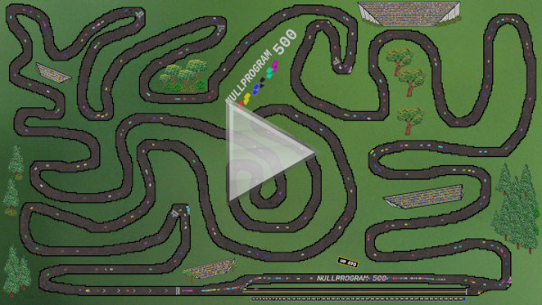
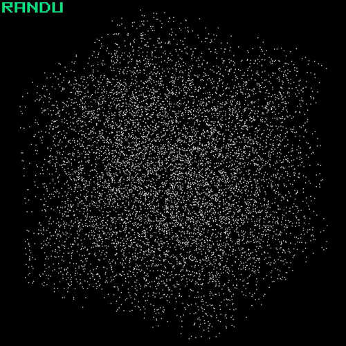
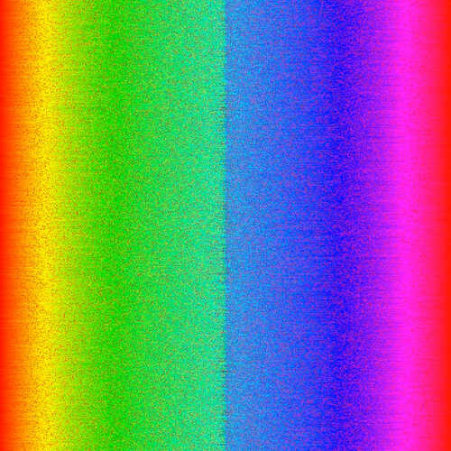
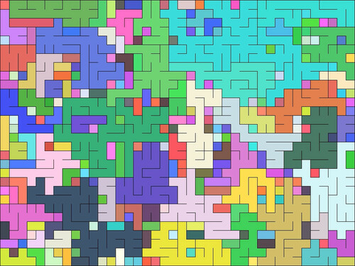
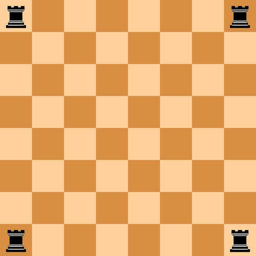
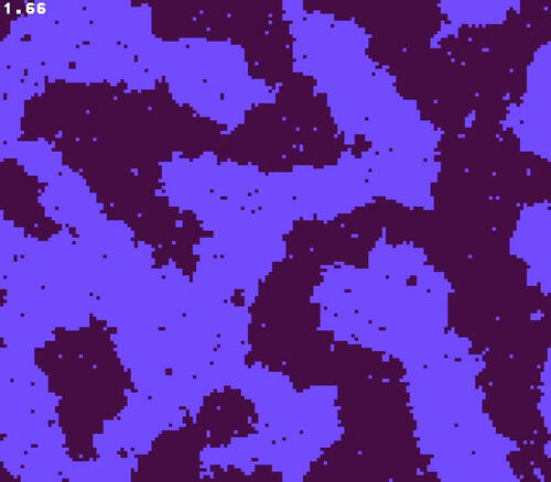
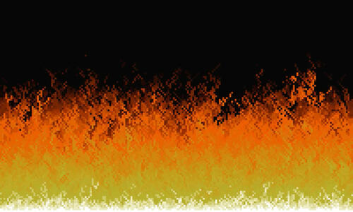
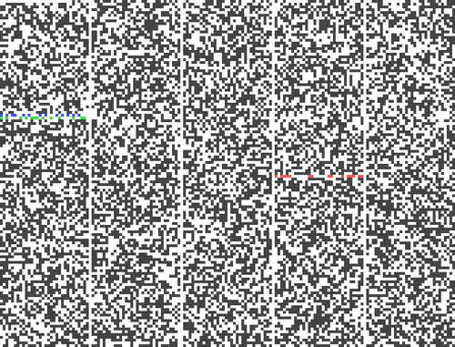
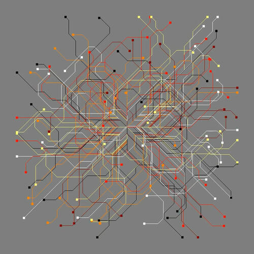
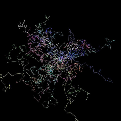
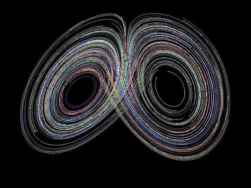
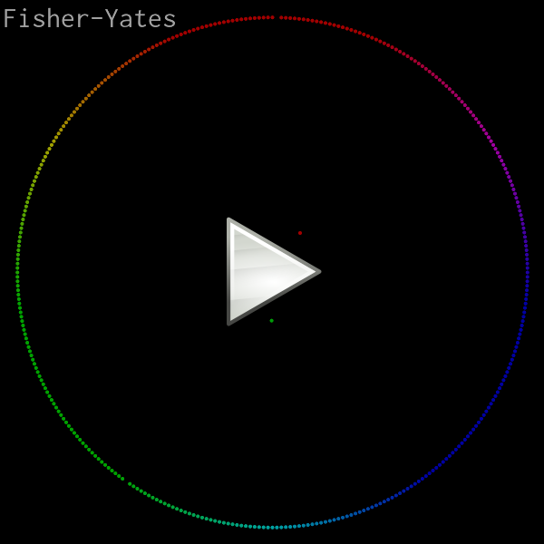
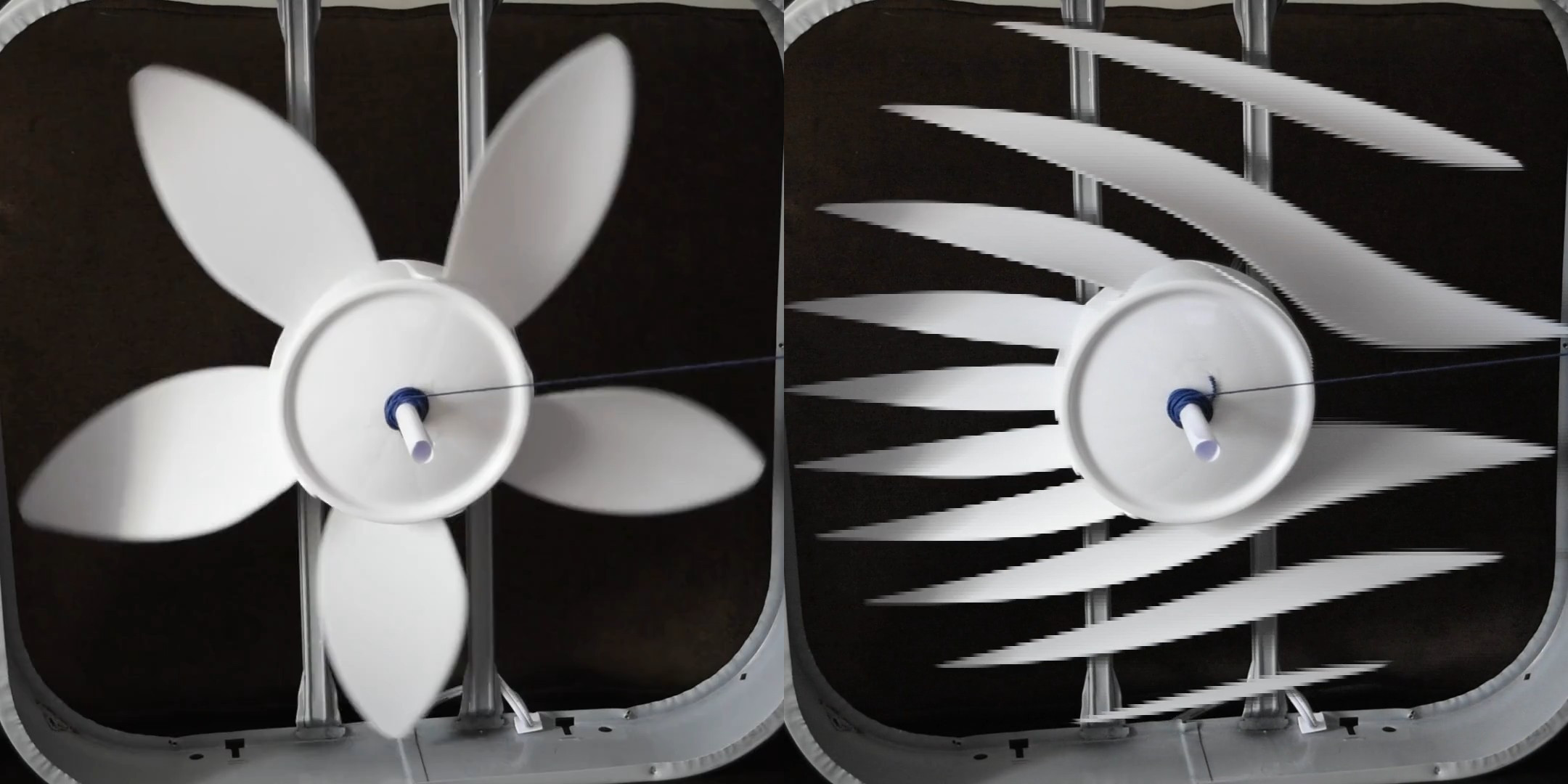
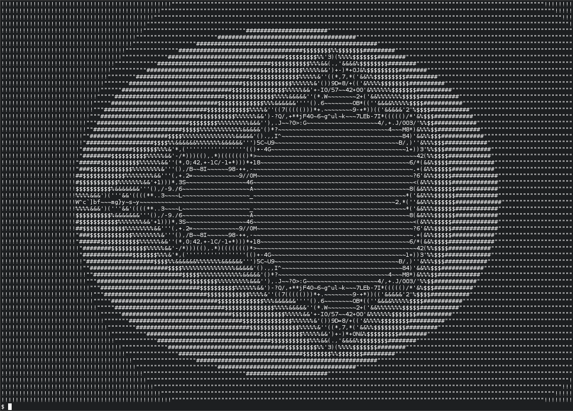
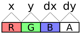
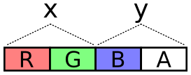
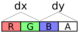
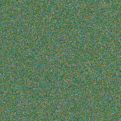
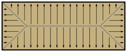
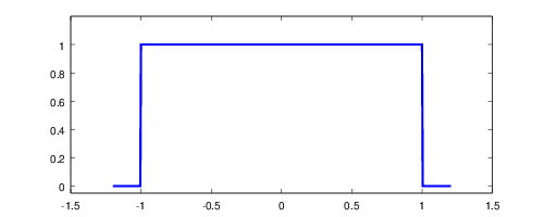
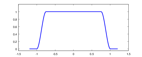
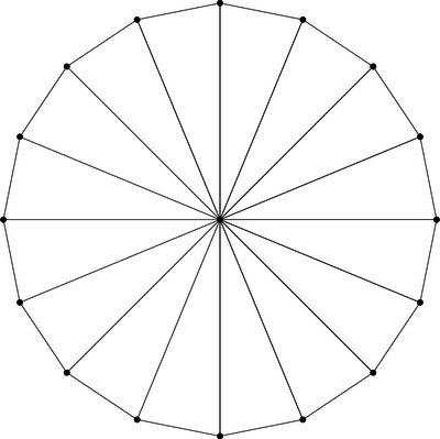
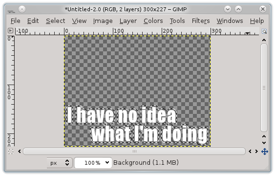
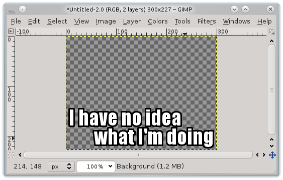
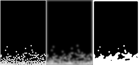
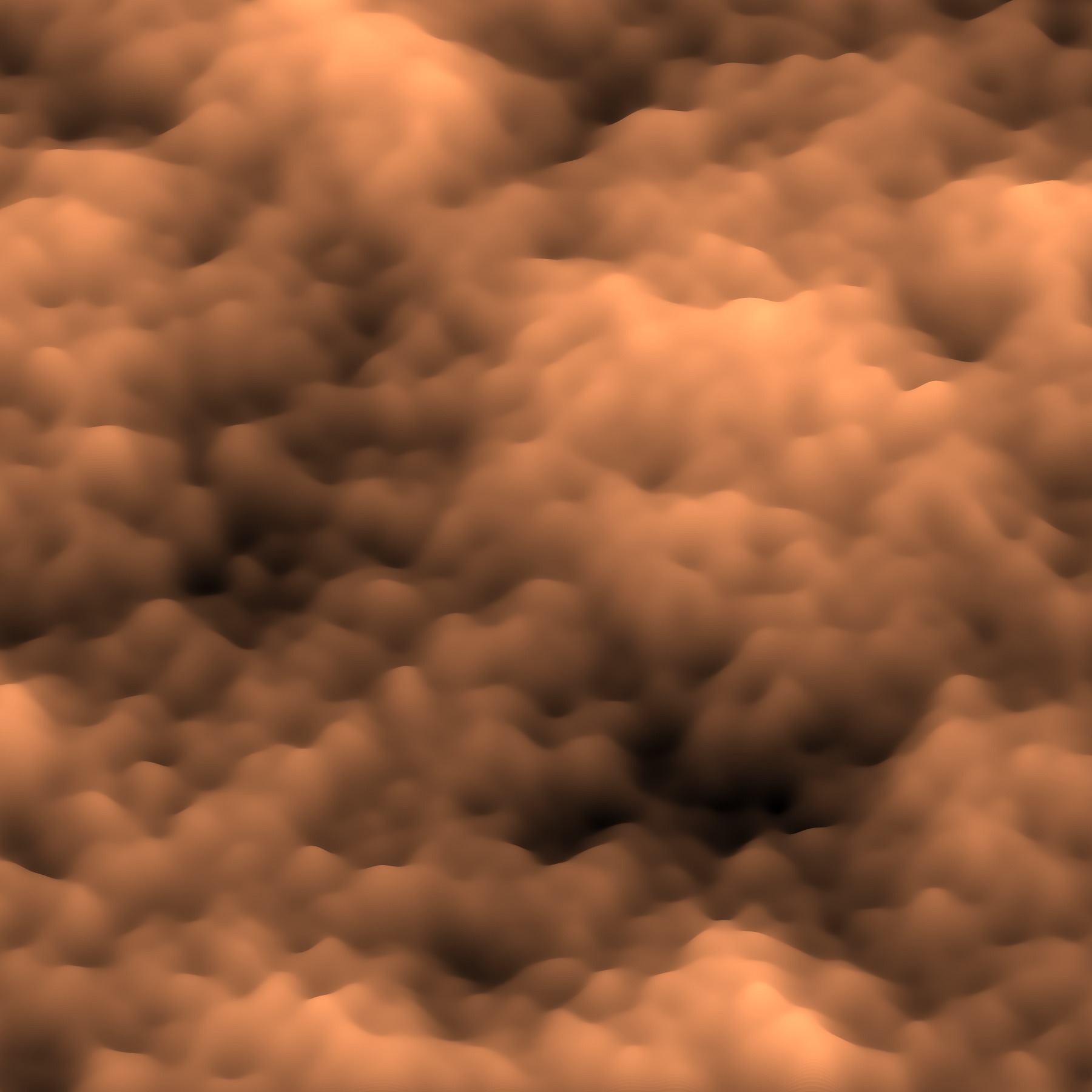
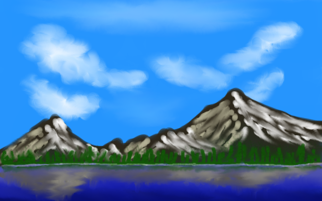
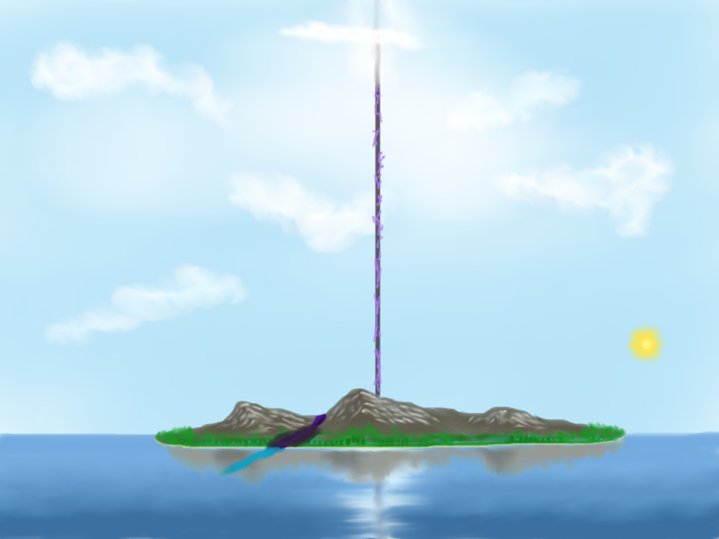
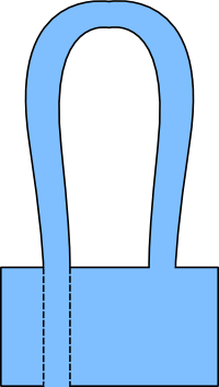
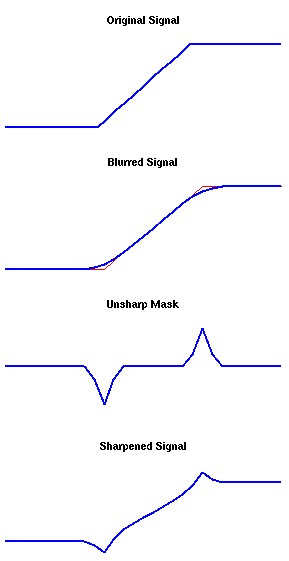
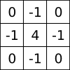