<?xml version="1.0" encoding="UTF-8"?>
<feed xmlns="http://www.w3.org/2005/Atom">

  <title>Articles tagged octave at null program</title>
  <link rel="alternate" type="text/html"
        href="https://nullprogram.com/tags/octave/"/>
  <link rel="self" type="application/atom+xml"
        href="https://nullprogram.com/tags/octave/feed/"/>
  <updated>2026-04-09T13:25:45Z</updated>
  <id>urn:uuid:ae7db2fb-eac3-4621-bae3-876c87011475</id>

  <author>
    <name>Christopher Wellons</name>
    <uri>https://nullprogram.com</uri>
    <email>wellons@nullprogram.com</email>
  </author>


  <entry>
    <title>Perlin Noise With Octave, Java, and OpenCL</title>
    <link rel="alternate" type="text/html" href="https://nullprogram.com/blog/2012/06/03/"/>
    <id>urn:uuid:830cc950-634a-3661-135a-b932c8c5399e</id>
    <updated>2012-06-03T00:00:00Z</updated>
    <category term="java"/><category term="c"/><category term="octave"/><category term="video"/>
    <content type="html">
      <![CDATA[<p>I recently discovered that I’m an idiot and that my
<a href="/blog/2007/11/20/">old Perlin noise post</a> was not actually describing
Perlin noise at all, but fractional Brownian motion. Perlin noise is
slightly more complicated but much more powerful. To learn the correct
algorithm, I wrote three different implementations
(<a href="https://github.com/skeeto/perlin-noise">perlin-noise</a>).</p>

<div class="language-plaintext highlighter-rouge"><div class="highlight"><pre class="highlight"><code>git clone git://github.com/skeeto/perlin-noise.git
</code></pre></div></div>

<p>In short, Perlin noise is based on a grid of randomly-generated
gradient vectors which describe how the arbitrarily-dimensional
“surface” is sloped at that point. The noise at the grid points is
always 0, though you’d never know it. When sampling the noise at some
point between grid points, a weighted interpolation of the surrounding
gradient vectors is calculated. Vectors are reduced to a single noise
value by dot product.</p>

<p>Rather than waste time trying to explain it myself, I’ll link to an
existing, great tutorial: <a href="https://web.archive.org/web/20150304163452/http://webstaff.itn.liu.se/~stegu/TNM022-2005/perlinnoiselinks/perlin-noise-math-faq.html">The Perlin noise math FAQ</a>. There’s
also the original presentation by Ken Perlin, <a href="(http://www.noisemachine.com/talk1/)">Making Noise</a>,
which is more concise but harder to grok.</p>

<p>When making my own implementation, I started by with Octave. It’s my
“go to language” for creating a prototype when I’m doing something
with vectors or matrices since it has the most concise syntax for
these things. I wrote a two-dimensional generator and it turned out to
be a lot simpler than I thought it would be!</p>

<ul>
  <li><a href="https://github.com/skeeto/perlin-noise/blob/master/octave/perlin2d.m">perlin2d.m</a></li>
</ul>

<p>Because it’s 2D, there are four surrounding grid points to consider
and these are all hard-coded. This leads to an interesting property:
there are no loops. The code is entirely vectorized, which makes it
quite fast. It actually keeps up with my generalized Java solution
(next) when given a grid of points, such as from <code class="language-plaintext highlighter-rouge">meshgrid()</code>.</p>

<p>
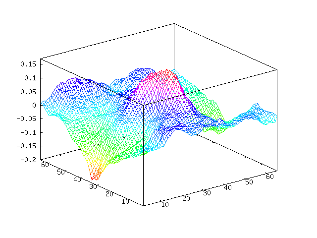
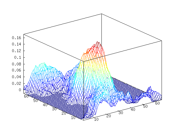
The grid gradient vectors are generated on the fly by a hash
function. The integer x and y positions of the point are hashed using
a bastardized version of Robert Jenkins’ 96 bit mix function (the one
I used in my <a href="/blog/2011/06/13/">infinite parallax starfield</a>) to
produce a vector. This turned out to be the trickiest part to write,
because any weaknesses in the hash function become very apparent in
the resulting noise.</p>

<p>
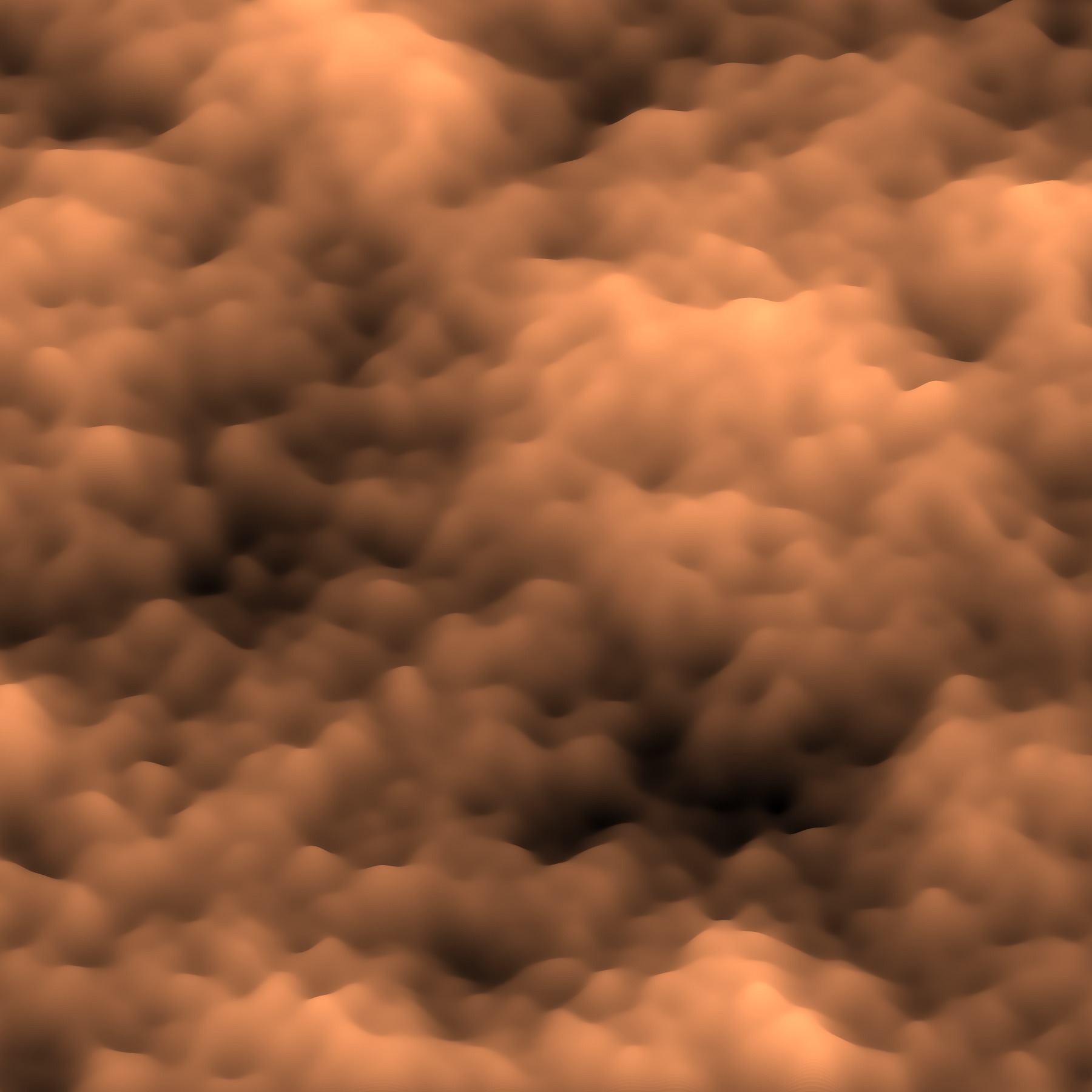
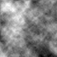
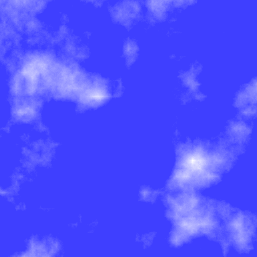
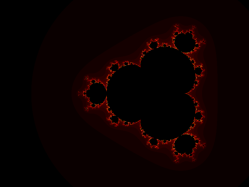
Using Octave, this took two seconds to generate on my laptop. You
can’t really tell by looking at it, but, as with all Perlin noise,
there is actually a grid pattern.
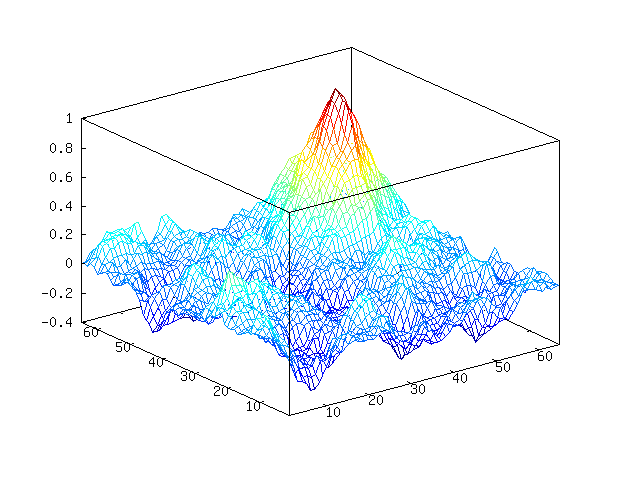
</p>

<p><img src="/img/noise/octave-perlin2d.png" alt="" /></p>

<p>I then wrote a generalized version, <code class="language-plaintext highlighter-rouge">perlin.m</code>, that can generate
arbitrarily-dimensional noise. This one is a lot shorter, but it’s not
vectorized, can only sample one point at a time, and is incredibly
slow. For a hash function, I use Octave’s <code class="language-plaintext highlighter-rouge">hashmd5()</code>, so this one
won’t work in Matlab (which provides no hash function
whatsoever). However, it <em>is</em> a lot shorter!</p>

<div class="language-matlab highlighter-rouge"><div class="highlight"><pre class="highlight"><code><span class="c1">%% Returns the Perlin noise value for an arbitrary point.</span>
<span class="k">function</span> <span class="n">v</span> <span class="o">=</span> <span class="n">perlin</span><span class="p">(</span><span class="n">p</span><span class="p">)</span>
  <span class="n">v</span> <span class="o">=</span> <span class="mi">0</span><span class="p">;</span>
  <span class="c1">%% Iterate over each corner</span>
  <span class="k">for</span> <span class="n">dirs</span> <span class="o">=</span> <span class="p">[</span><span class="nb">dec2bin</span><span class="p">(</span><span class="mi">0</span><span class="p">:(</span><span class="mi">2</span> <span class="o">^</span> <span class="nb">length</span><span class="p">(</span><span class="n">p</span><span class="p">)</span> <span class="o">-</span> <span class="mi">1</span><span class="p">))</span> <span class="o">-</span> <span class="mi">48</span><span class="p">]</span><span class="o">'</span>
    <span class="n">q</span> <span class="o">=</span> <span class="nb">floor</span><span class="p">(</span><span class="n">p</span><span class="p">)</span> <span class="o">+</span> <span class="n">dirs</span><span class="s1">'; % This iteration'</span><span class="n">s</span> <span class="n">corner</span>
    <span class="n">g</span> <span class="o">=</span> <span class="n">qgradient</span><span class="p">(</span><span class="n">q</span><span class="p">);</span> <span class="c1">% This corner's gradient</span>
    <span class="n">m</span> <span class="o">=</span> <span class="nb">dot</span><span class="p">(</span><span class="n">g</span><span class="p">,</span> <span class="n">p</span> <span class="o">-</span> <span class="n">q</span><span class="p">);</span>
    <span class="n">t</span> <span class="o">=</span> <span class="mf">1.0</span> <span class="o">-</span> <span class="nb">abs</span><span class="p">(</span><span class="n">p</span> <span class="o">-</span> <span class="n">q</span><span class="p">);</span>
    <span class="n">v</span> <span class="o">+=</span> <span class="n">m</span> <span class="o">*</span> <span class="nb">prod</span><span class="p">(</span><span class="mi">3</span> <span class="o">*</span> <span class="n">t</span> <span class="o">.^</span> <span class="mi">2</span> <span class="o">-</span> <span class="mi">2</span> <span class="o">*</span> <span class="n">t</span> <span class="o">.^</span> <span class="mi">3</span><span class="p">);</span>
  <span class="k">end</span>
<span class="k">end</span>

<span class="c1">%% Return the gradient at the given grid point.</span>
<span class="k">function</span> <span class="n">v</span> <span class="o">=</span> <span class="n">qgradient</span><span class="p">(</span><span class="n">q</span><span class="p">)</span>
  <span class="n">v</span> <span class="o">=</span> <span class="nb">zeros</span><span class="p">(</span><span class="nb">size</span><span class="p">(</span><span class="n">q</span><span class="p">));</span>
  <span class="k">for</span> <span class="n">i</span> <span class="o">=</span> <span class="mi">1</span><span class="p">:</span><span class="nb">length</span><span class="p">(</span><span class="n">q</span><span class="p">);</span>
      <span class="n">v</span><span class="p">(</span><span class="n">i</span><span class="p">)</span> <span class="o">=</span> <span class="n">hashmd5</span><span class="p">([</span><span class="n">i</span> <span class="n">q</span><span class="p">])</span> <span class="o">*</span> <span class="mf">2.0</span> <span class="o">-</span> <span class="mf">1.0</span><span class="p">;</span>
  <span class="k">end</span>
<span class="k">end</span>
</code></pre></div></div>

<p>
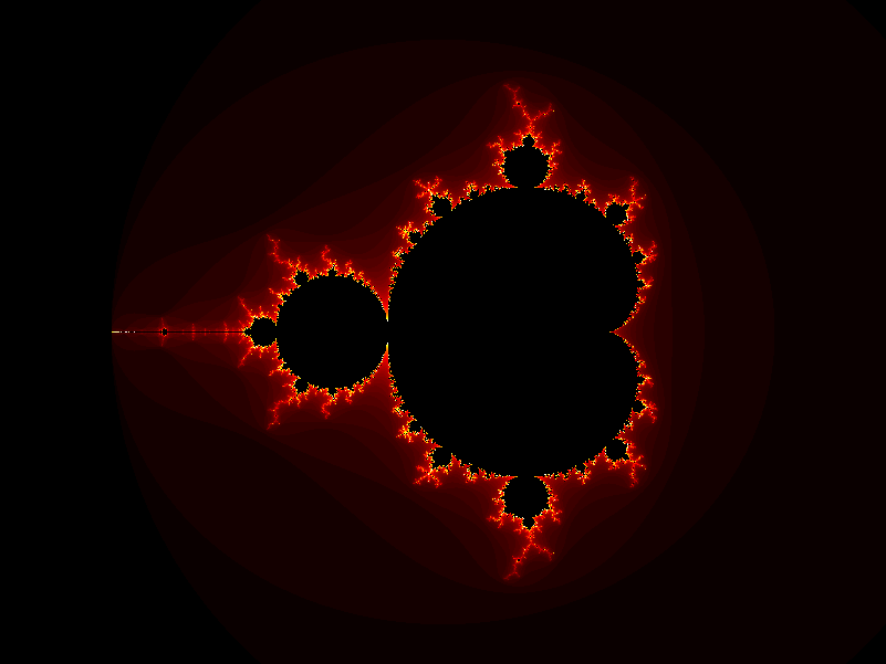
It took Octave an entire day to generate this “fire” video, which is
ridiculously long. An old graphics card could probably do this in real
time.</p>

<video src="https://nullprogram.s3.amazonaws.com/noise/fire.webm" width="300" height="300" controls="controls">
  Your browser doesn't support HTML5 video with WebM. :-(
</video>

<p>This was produced by viewing a slice of 3D noise. For animation, the
viewing area moves in two dimensions (z and y). One dimension makes
the fire flicker, the other makes it look like it’s rising. A simple
gradient was applied to the resulting noise to fade away towards the
top.</p>

<p>I wanted to achieve this same effect faster, so next I made a
generalized Java implementation, which is the bulk of the
repository. I wrote my own Vector class (completely unlike Java’s
depreciated Vector but more like Apache Commons Math’s RealVector), so
it looks very similar to the Octave version. It’s much, much faster
than the generalized Octave version. It doesn’t use a hash function
for gradients — instead randomly generating them as needed and
keeping track of them for later with a Map.</p>

<p>I wanted to go faster yet, so next I looked at OpenCL for the first
time. OpenCL is an API that allows you to run C-like programs on your
graphics processing unit (GPU), among other things. I was sticking to
Java so I used <a href="http://www.lwjgl.org/">lwjgl</a>’s OpenCL bindings. In
order to use this code you’ll need an OpenCL implementation available
on your system, which, unfortunately, is usually proprietary. My
OpenCL noise generator only generates 3D noise.</p>

<p>Why use the GPU? GPUs have a highly-parallel structure that makes them
faster than CPUs at processing large blocks of data in parallel. This
is really important when it comes to computer graphics, but it can be
useful for other purposes as well, like generating Perlin noise.</p>

<p>I had to change my API a little to make this effective. Before, to
generate noise samples, I passed points in individually to
PerlinNoise. To properly parallelize this for OpenCL, an entire slice
is specified by setting its width, height, step size, and
z-level. This information, along with pre-computed grid gradients, is
sent to the GPU.</p>

<ul>
  <li><a href="https://github.com/skeeto/perlin-noise/blob/opencl/src/com/nullprogram/noise/perlin3d.cl">perlin3d.cl</a></li>
</ul>

<p>This is all in the <code class="language-plaintext highlighter-rouge">opencl</code> branch in the repository. When run, it
will produce a series of slices of 3D noise in a manner similar to the
fire example above. For comparison, it will use the CPU by default,
generating a series of <code class="language-plaintext highlighter-rouge">simple-*.png</code>. Give the program one argument,
“opencl”, and it will use OpenCL instead, generating a series of
<code class="language-plaintext highlighter-rouge">opencl-*.png</code>. You should notice a massive increase in speed when
using OpenCL. In fact, it’s even faster than this. The vast majority
of the time is spent creating these output PNG images. When I disabled
image output for both, OpenCL was 200 times faster than the
(single-core) CPU implementation, still spending a significant amount
of time just loading data off the GPU.</p>

<p>And finally, I turned the OpenCL output into a video,</p>

<video src="https://nullprogram.s3.amazonaws.com/noise/opencl.webm" width="400" height="400" controls="controls">
  Your browser doesn't support HTML5 video with WebM. :-(
</video>

<p>That’s pretty cool!</p>

<p>I still don’t really have a use for Perlin noise, especially not under
constraints that require I use OpenCL to generate it. The big thing I
got out of this project was my first experience with OpenCL, something
that really <em>is</em> useful at work.</p>

]]>
    </content>
  </entry>


  <entry>
    <title>Lisp Let in GNU Octave</title>
    <link rel="alternate" type="text/html" href="https://nullprogram.com/blog/2012/02/08/"/>
    <id>urn:uuid:05e5318e-0cf4-3d80-4bf5-da695dbe9e47</id>
    <updated>2012-02-08T00:00:00Z</updated>
    <category term="octave"/><category term="trick"/><category term="lisp"/><category term="media"/><category term="math"/><category term="video"/>
    <content type="html">
      <![CDATA[<p>In <a href="/blog/2011/01/30/">BrianScheme</a>, the standard Lisp binding form <code class="language-plaintext highlighter-rouge">let</code> isn’t a
special form. That is, it’s not a hard-coded language feature, or
<em>special form</em>. It’s built on top of <code class="language-plaintext highlighter-rouge">lambda</code>. In any lexically-scoped
Lisp, the expression,</p>

<div class="language-cl highlighter-rouge"><div class="highlight"><pre class="highlight"><code><span class="p">(</span><span class="k">let</span> <span class="p">((</span><span class="nv">x</span> <span class="mi">10</span><span class="p">)</span>
      <span class="p">(</span><span class="nv">y</span> <span class="mi">20</span><span class="p">))</span>
  <span class="p">(</span><span class="nb">*</span> <span class="mi">10</span> <span class="mi">20</span><span class="p">))</span>
</code></pre></div></div>

<p>Can also be written as,</p>

<div class="language-cl highlighter-rouge"><div class="highlight"><pre class="highlight"><code><span class="p">((</span><span class="k">lambda</span> <span class="p">(</span><span class="nv">x</span> <span class="nv">y</span><span class="p">)</span>
   <span class="p">(</span><span class="nb">*</span> <span class="nv">x</span> <span class="nv">y</span><span class="p">))</span>
 <span class="mi">10</span> <span class="mi">20</span><span class="p">)</span>
</code></pre></div></div>

<p>BrianScheme’s <code class="language-plaintext highlighter-rouge">let</code> is just a macro that transforms into a lambda
expression. This is also what made it so important to implement lambda
lifting, to optimize these otherwise-expensive forms.</p>

<p>It’s possible to achieve a similar effect in GNU Octave (but not
Matlab, due to <a href="/blog/2008/08/29/">its flawed parser design</a>). The language permits
simple lambda expressions, much like Python.</p>

<div class="language-matlab highlighter-rouge"><div class="highlight"><pre class="highlight"><code><span class="o">&gt;</span> <span class="n">f</span> <span class="o">=</span> <span class="o">@</span><span class="p">(</span><span class="n">x</span><span class="p">)</span> <span class="n">x</span> <span class="o">+</span> <span class="mi">10</span><span class="p">;</span>
<span class="o">&gt;</span> <span class="n">f</span><span class="p">(</span><span class="mi">4</span><span class="p">)</span>
<span class="nb">ans</span> <span class="o">=</span> <span class="mi">14</span>
</code></pre></div></div>

<p>It can be used to create a scope in a language that’s mostly devoid of
scope. For example, I can avoid assigning a value to a temporary
variable just because I need to use it in two places. This one-liner
generates a random 3D unit vector.</p>

<div class="language-matlab highlighter-rouge"><div class="highlight"><pre class="highlight"><code><span class="p">(</span><span class="o">@</span><span class="p">(</span><span class="n">v</span><span class="p">)</span> <span class="n">v</span> <span class="p">/</span> <span class="nb">norm</span><span class="p">(</span><span class="n">v</span><span class="p">))(</span><span class="nb">randn</span><span class="p">(</span><span class="mi">1</span><span class="p">,</span> <span class="mi">3</span><span class="p">))</span>
</code></pre></div></div>

<p>The anonymous function is called inside the same expression where it’s
created. In practice, doing this is stupid. It’s confusing and there’s
really nothing to gain by being clever, doing it in one line instead
of two. Most importantly, there’s no macro system that can turn this
into a new language feature. <em>However</em>, I enjoyed using this technique
to create a one-liner that generates <code class="language-plaintext highlighter-rouge">n</code> random unit vectors.</p>

<div class="language-matlab highlighter-rouge"><div class="highlight"><pre class="highlight"><code><span class="n">n</span> <span class="o">=</span> <span class="mi">1000</span><span class="p">;</span>
<span class="n">p</span> <span class="o">=</span> <span class="p">(</span><span class="o">@</span><span class="p">(</span><span class="n">v</span><span class="p">)</span> <span class="n">v</span> <span class="o">.</span><span class="p">/</span> <span class="nb">repmat</span><span class="p">(</span><span class="nb">sqrt</span><span class="p">(</span><span class="nb">sum</span><span class="p">(</span><span class="nb">abs</span><span class="p">(</span><span class="n">v</span><span class="p">)</span> <span class="o">.^</span> <span class="mi">2</span><span class="p">,</span> <span class="mi">2</span><span class="p">)),</span> <span class="mi">1</span><span class="p">,</span> <span class="mi">3</span><span class="p">))(</span><span class="nb">randn</span><span class="p">(</span><span class="n">n</span><span class="p">,</span> <span class="mi">3</span><span class="p">));</span>
</code></pre></div></div>

<p>Why was I doing this? I was using the Monte Carlo method to
double-check my solution to <a href="http://godplaysdice.blogspot.com/2011/12/geometric-probability-problem.html">this math problem</a>:</p>

<blockquote>
  <p>What is the average straight line distance between two points on a
sphere of radius 1?</p>
</blockquote>

<p>I was also demonstrating to <a href="http://devrand.org/">Gavin</a> that simply choosing two
<em>angles</em> is insufficient, because the points the angles select are not
evenly distributed over the surface of the sphere. I generated this
video, where the poles are clearly visible due to the uneven selection
by two angles.</p>

<video src="https://s3.amazonaws.com/nullprogram/sphere/sphere-dark.webm" controls="controls" height="340" width="340">
</video>

<p>This took hours to render with gnuplot! Here are stylized versions:
<a href="https://s3.amazonaws.com/nullprogram/sphere/dark.html">Dark</a> and <a href="https://s3.amazonaws.com/nullprogram/sphere/light.html">Light</a>.</p>

]]>
    </content>
  </entry>


  <entry>
    <title>Silky Smooth Perlin Noise Surface</title>
    <link rel="alternate" type="text/html" href="https://nullprogram.com/blog/2012/01/19/"/>
    <id>urn:uuid:3b93a02f-93e1-3221-2405-58a83127968e</id>
    <updated>2012-01-19T00:00:00Z</updated>
    <category term="octave"/><category term="math"/><category term="media"/>
    <content type="html">
      <![CDATA[<p>At work I’ve recently been generating
<a href="http://en.wikipedia.org/wiki/Viewshed">viewsheds</a> over
<a href="http://en.wikipedia.org/wiki/DTED">DTED</a> sets. Earlier this week I
was asked to give an informal presentation on what I was doing. I
wanted some terrain that demonstrated some key features, such as
vision being occluded by hills of varying heights. Rather than search
through the available DTED files for something good, I opted for
generating my own terrain, using an old trick of mine:
<a href="/blog/2007/11/20/">my noise “cloud” generator</a>. That’s a lesson in
the usefulness of maintaining a blog. The useful things you learn and
create are easy to revisit years later!</p>

<p>I generated some noise, looked at it with <code class="language-plaintext highlighter-rouge">surf()</code>, and repeated until
I found something useful. (<em>Update June 2012:</em> the function is called
<code class="language-plaintext highlighter-rouge">perlin()</code> but it’s not actually Perlin noise.)</p>

<div class="language-matlab highlighter-rouge"><div class="highlight"><pre class="highlight"><code><span class="n">m</span> <span class="o">=</span> <span class="n">perlin</span><span class="p">(</span><span class="mi">1024</span><span class="p">);</span>
<span class="nb">surf</span><span class="p">(</span><span class="n">m</span><span class="p">);</span>
</code></pre></div></div>

<p>The generated terrain is really quite rough, so I decided to smooth it
out by <a href="/blog/2008/02/22/">convolving it with a 2-dimensional Gaussian kernel</a>.</p>

<div class="language-matlab highlighter-rouge"><div class="highlight"><pre class="highlight"><code><span class="n">k</span> <span class="o">=</span> <span class="n">fspecial</span><span class="p">(</span><span class="s1">'gaussian'</span><span class="p">,</span> <span class="mi">9</span><span class="p">);</span>
<span class="n">ms</span> <span class="o">=</span> <span class="nb">conv2</span><span class="p">(</span><span class="n">m</span><span class="p">,</span> <span class="n">k</span><span class="p">,</span> <span class="s1">'same'</span><span class="p">);</span>
</code></pre></div></div>

<p>It still wasn’t smooth enough. So I repeated the process a bit,</p>

<div class="language-matlab highlighter-rouge"><div class="highlight"><pre class="highlight"><code><span class="k">for</span> <span class="n">i</span> <span class="o">=</span> <span class="mi">1</span><span class="p">:</span><span class="mi">10</span>
    <span class="n">ms</span> <span class="o">=</span> <span class="nb">conv2</span><span class="p">(</span><span class="n">ms</span><span class="p">,</span> <span class="n">k</span><span class="p">,</span> <span class="s1">'same'</span><span class="p">);</span>
<span class="k">end</span>
</code></pre></div></div>

<p>Perfect! I used that for my presentation. However, I was having fun
and decided to experiment more with this. I filtered it again another
1000 times and generated a <code class="language-plaintext highlighter-rouge">surf()</code> plot with a high-resolution
colormap — the default colormap size caused banding.</p>

<div class="language-matlab highlighter-rouge"><div class="highlight"><pre class="highlight"><code><span class="nb">colormap</span><span class="p">(</span><span class="nb">copper</span><span class="p">(</span><span class="mi">1024</span><span class="p">));</span>
<span class="nb">surf</span><span class="p">(</span><span class="n">ms</span><span class="p">,</span> <span class="s1">'EdgeAlpha'</span><span class="p">,</span> <span class="mi">0</span><span class="p">);</span>
<span class="nb">axis</span><span class="p">(</span><span class="s1">'equal'</span><span class="p">);</span>
</code></pre></div></div>

<p>It produced this beautiful result!</p>

<p><a href="/img/noise/silk-perlin-surface.jpg"><img src="/img/noise/silk-perlin-surface-thumb.jpg" alt="" /></a></p>

<p>I think it looks like a photograph from a high-powered microscope, or
maybe the turbulent surface of some kind of creamy beverage being
stirred.</p>

<p>At work when I need something Matlab-ish, I use Octave about half the
time and Matlab the other half. In this case, I was using
Matlab. Octave doesn’t support the <code class="language-plaintext highlighter-rouge">EdgeAlpha</code> property, nor the
<code class="language-plaintext highlighter-rouge">viewshed()</code> function that I needed for my work. Matlab currently
makes much prettier plots than Octave.</p>
]]>
    </content>
  </entry>


  <entry>
    <title>A GNU Octave Feature</title>
    <link rel="alternate" type="text/html" href="https://nullprogram.com/blog/2008/08/29/"/>
    <id>urn:uuid:a8aec192-263a-38d3-5d0d-86824c93fd4f</id>
    <updated>2008-08-29T00:00:00Z</updated>
    <category term="octave"/><category term="rant"/><category term="lang"/>
    <content type="html">
      <![CDATA[<!-- 29 August 2008 -->
<p>
At work they recently moved me to a new project. It is a Matlab-based
data analysis thing. I haven't really touched Matlab in over a year
(the last time I used Matlab at work), and, instead, use GNU Octave at
home when the language is appropriate. I got so used to Octave that I
found a pretty critical feature missing from Matlab's implementation:
treat an expression as if it were of the type of its output.
</p>
<p>
Let's say we want to index into the result of a function. Take, for
example, the magic square function, <code>magic()</code>. This spits
out a
<a href="http://en.wikipedia.org/wiki/Magic_square">magic square</a>
of the given size. In Octave we can generate a 4x4 magic square and
chop out the middle 2x2 portion in one line.
</p>
<pre>
octave> magic(4)(2:3,2:3)
ans =

   11   10
    7    6
</pre>
<p>
Or more possibly clearly,
</p>
<pre>
octave> [magic(4)](2:3,2:3)
ans =

   11   10
    7    6
</pre>
<p>
Try this in Matlab and you will get a big, fat error. You have to
assign the magic square to a temporary variable to do the same
thing. I kept trying to do this sort of thing in Matlab and was
thinking to myself, "I <i>know</i> I can do this somehow!". Nope, I
was just used to having Octave.
</p>
<p>
Where this really shows is when you want to reshape a matrix into a
nice, simple vector. If you have a matrix <code>M</code> and want to
count the number of NaN's it has, you can't just apply
the <code>sum()</code> function over <code>isnan()</code> because it
only does sums of columns. You can get around this with a special
index, <code>(:)</code>.
</p>
<p>
So, to sum all elements in <code>M</code> directly,
</p>
<pre>
octave> sum(M(:))
</pre>
<p>
In Octave, to count NaN's with <code>isnan()</code>,
</p>
<pre>
octave> sum(isnan(M)(:))
</pre>
<p>
Again, Matlab won't let you index the result of <code>isnan()</code>
directly. Stupid. I guess the Matlab way to do this is to
apply <code>sum()</code> twice.
</p>
<p> Every language I can think of handles this properly. C, C++, Perl,
Ruby, etc. It is strange that Matlab itself doesn't have it. Score one
more for Octave.
</p>
]]>
    </content>
  </entry>


  <entry>
    <title>Linear Spatial Filters with GNU Octave</title>
    <link rel="alternate" type="text/html" href="https://nullprogram.com/blog/2008/02/22/"/>
    <id>urn:uuid:e3b9e7a9-5669-3173-f84d-d8af0d8f8be4</id>
    <updated>2008-02-22T00:00:00Z</updated>
    <category term="octave"/><category term="tutorial"/>
    <content type="html">
      <![CDATA[<!-- 22 February 2008 -->
<p>
  <a href="/img/spatial/image-test.svg">
    <img src="/img/spatial/image-test-small.png" alt=""/>
  </a>
  <img src="/img/spatial/image-test-small-ave.png" alt=""/>
  <img src="/img/spatial/image-test-small-gauss.png" alt=""/>
  <img src="/img/spatial/image-test-small-edge.png" alt=""/>
</p>
<p style="font-style: italic;">
I have gotten several e-mails lately about using GNU Octave. One
specifically was about blurring images in Octave. In response, I am
writing this in-depth post to cover spatial filters, and how to use
them in GNU Octave (a free implementation of the Matlab programming
language). This should be the sort of information you would find near
the beginning of an introductory digital image processing textbook,
but written out more simply. In the future, I will probably be writing
a post covering non-linear spatial and/or frequency domain filters in
Octave.
</p>
<p style="font-style: italic;">
If you want to follow along in Octave, I strongly recommend that you
upgrade to the new Octave 3.0. It is considered stable, but differs
significantly from Octave 2.1, which many people may be used to. You
will also need to install
the <a href="http://octave.sourceforge.net/image/index.html"> image
processing package</a>
from <a href="http://octave.sourceforge.net/">Octave-Forge.</a> To get
help with any Octave function, just type <code>help
&lt;function&gt;</code>.
</p>
<p>
The most common linear spatial image filtering
involves <a href="http://en.wikipedia.org/wiki/Convolution">
convolving</a> a <i>filter mask</i>, sometimes called a <i>convolution
kernel</i>, over an image, which is a two-dimensional matrix. In the
case of an <abbr title="Red, Green, Blue">RGB</abbr> color
image, the image is actually composed of three two-dimensional
grayscale images, each representing a single color, where each is
convolved with the filter mask separately.
</p>
<p>
Convolution is sliding a mask over an image. The new value at the
mask's position is the sum of the value of each element of the mask
multiplied by the value of the image at that position. For an example,
let's start with 1-dimensional convolution. Define a mask,
</p>
<pre>
5 3 2 4 8
</pre>
<p>
The 2 is the anchor for the mask. Define an image,
</p>
<pre>
0 0 1 2 1 0 0
</pre>
<p>
As we convolve, the mask will extend beyond the image at the
edges. One way to handle this is to pad the image with 0's. We start
by placing the mask at the left edge. (zero-padding is underlined)
</p>
<pre>
Mask:   5 3 2 4 8
Image:  <b>0 0</b> 0 0 1 2 1 0 0
</pre>
<p>
The first output value is 8, as every other element of the mask is
multiplied by zero.
</p>
<pre>
Output: 8 x x x x x x
</pre>
<p>
Now, slide the mask over by one position,
</p>
<pre>
Mask:   5 3 2 4 8
Image:  <b>0</b> 0 0 1 2 1 0 0
</pre>
<p>
The output here is 20, because 8*2 + 4*1 = 20;
</p>
<pre>
Output: 8 20 x x x x x
</pre>
<p>
If we continue sliding the mask along, the output becomes,
</p>
<pre>
Output: 8 20 18 11 13 13 5
</pre>
<p>
Here is the correlation done in Octave interactively,
(<code>filter2()</code> is the correlation function).
</p>
<pre>
octave> filter2([5 3 2 4 8], [0 0 1 2 1 0 0])
ans =

    8   20   18   11   13   13    5

</pre>
<p>
The same thing happens in two-dimensional convolution, with the mask
moving in the vertical direction as well, so that each element in the
image is covered.
</p>
<p>
  <img src="/img/spatial/draw-filter.png" alt=""/>
</p>
<p>
Sometimes you will hear this described as correlation
(Octave's <code>filter2</code>) or convolution
(Octave's <code>conv2</code>). The only difference between these
operations is that in convolution the filter masked is rotated 180
degrees. Whoop-dee-doo. Most of the time your filter is probably
symmetrical anyway. So, don't worry much about the difference between
these two. Especially in Octave, where rotating a matrix is easy
(see <code>rot90()</code>).
</p>
<p>
Now that we know convolution, let's introduce the sample image we will
be using. I carefully put this together
in <a href="http://www.inkscape.org/">Inkscape</a>, which should give
us a nice scalable test image. When converting to a raster format,
there is a bit of unwanted anti-aliasing going on (couldn't find a way
to turn that off), but it is minimal.
</p>
<p>
  <a href="/img/spatial/image-test.svg">
    <img src="/img/spatial/image-test.png" alt=""/>
  </a>
</p>
<p>
Save that image (the PNG file, not the linked SVG file) where you can
get to it in Octave. Now, let's load the image into Octave
using <code>imread()</code>.
</p>
<pre>
m = imread("image-test.png");
</pre>
<p>
The image is a grayscale image, so it has only one layer. The size
of <code>m</code> should be 300x300. You can check this like so (note
the lack of semicolon so we can see the output),
</p>
<pre>
size(m)
</pre>
<p>
You can view the image stored in <code>m</code>
with <code>imshow</code>. It doesn't care about the image dimensions
or size, so until you resize the plot window, it will probably be
stretched.
</p>
<pre>
imshow(m);
</pre>
<p>
Now, let's make an extremely simple 5x5 filter mask.
</p>
<pre>
f = ones(5) * 1/25
</pre>
<p>
Octave will show us what this matrix looks like.
</p>
<pre>
f =

   0.040000   0.040000   0.040000   0.040000   0.040000
   0.040000   0.040000   0.040000   0.040000   0.040000
   0.040000   0.040000   0.040000   0.040000   0.040000
   0.040000   0.040000   0.040000   0.040000   0.040000
   0.040000   0.040000   0.040000   0.040000   0.040000
</pre>
<p>
This filter mask is called an <i>averaging filter</i>. It simply
averages all the pixels around the image (think about how this works
out in the convolution). The effect will be to blur the image. It is
important to note here that the sum of the elements is 1 (or 100% if
you are thinking of averages). You can check it like so,
</p>
<pre>
sum(f(:))
</pre>
<p>
Now, to convolve the image with the filter mask
using <code>filter2()</code>.
</p>
<pre>
ave_m = filter2(f, m);
</pre>
<p>
You can view the filtered image again with <code>imshow()</code>
except that we need to first convert the image matrix to a matrix of
8-bit unsigned integers. It is kind of annoying that we need this, but
this is the way it is as of this writing.
</p>
<pre>
ave_m = uint8(ave_m);
imshow(ave_m);
</pre>
<p>
Or, we can save this image to a file
using <code>imwrite()</code>. Just like with <code>imshow()</code>,
you will first need to convert the image to <code>uint8</code>.
</p>
<pre>
imwrite("averaged.png", ave_m);
</pre>
<p>
  <img src="/img/spatial/image-test-ave.png" alt=""/>
</p>
<p>
There are a few things to notice about this image. First there is a
black border around the outside of the filtered image. This is due to
the zero-padding (black border) done by <code>filter2()</code>. The
border of the image had 0's averaged into them. Second, some parts of
the blurred image are "noisy". Here are some selected parts at 4x zoom.
</p>
<p>
  <img src="/img/spatial/ave-zoom.png" alt=""/>
</p>
<p>
Notice how the circle, and the "a" seem a little bit boxy? This is due
to the shape of our filter. Also notice that the blurring isn't as
smooth as it could be. This is because the filter itself isn't very
smooth. We'll fix both these problems with a new filter later.
</p>
<p>
First, here is how we can fix the border problem: we pad the image
with itself. Octave provides us three easy ways to do this. The first
is replicate padding: the padding outside the image is the same as the
nearest border pixel in the image. Circular padding: the padding from
from the opposite side of the image, as if it was wrapped. This would
be a good choice for a periodic image. Last, and probably the most
useful is symmetric: the padding is a mirror reflection of the image
itself.
</p>
<p>
To apply symmetric padding, we use the <code>padarray()</code>
function. We only want to pad the image by the amount that the mask
will "hang off". Let's pad the original image for a 9x9 filter, which
will hang off by 4 pixels each way,
</p>
<pre>
mpad = padarray(m, [4 4], "symmetric");
</pre>
<p>
Next, we will replace the averaging filter with a 2D Gaussian
distribution. The Gaussian, or normal, distribution has many wonderful
and useful properties (as a statistics professor I had once said,
anyone who considers themselves to be educated should know about the
normal distribution). One property that makes it useful is that if we
integrate the Gaussian distribution from minus infinity to infinity,
the result is 1. The easiest way to get the curve without having to
type in the equation is using <code>fspecial()</code>: a special
function for creating image filters.
</p>
<pre>
f_gauss = fspecial("gaussian", 9, 2);
</pre>
<p>
This creates a 9x9 Gaussian filter with variance 2. The variance
controls the effective size of the filter. Increasing the size of the
filter from 9 to 99 will actually have virtually no impact on the
final result. It just needs to be large enough to cover the curve. Six
times the variance covers over 99% of the curve, so for a variance of
2, a filter of size 7x7 (always make your filters odd in size) is
plenty. A larger filter means a longer convolution time. Here is what
the 9x9 filter looks like,
</p>
<p>
  <img src="/img/spatial/gauss2d.png" alt=""/>
</p>
<p>
And to filter with the Gaussian,
</p>
<pre>
gauss_m = filter2(f_gauss, mpad, "valid";
gauss_m = uint8(guass_m);
</pre>
<p>
Notice the extra argument <code>"valid"</code>? Since we padded the
image before filtering, we don't want this padding to be part of the
image result. <code>filter2()</code> normally returns an image of the
same size as the input image, but we only want the part that didn't
undergo (additional) zero-padding. The result is now the same size as
the original image, but without the messy border,
</p>
<p>
  <img src="/img/spatial/image-test-gauss.png" alt=""/>
</p>
<p>
Also, compare the result to the average filter above. See how much
smoother this image is? If you are interested in blurring an image,
you will generally want to go with a Gaussian filter like this.
</p>
<p>
Now I will let you in on a little shortcut. In Matlab, there is a
function called <code>imfilter</code> which does the padding and
filtering in one step. As of this writing, the Octave-Forge image
package doesn't officially include this function, but it is there in
the source repository now, meaning that it will probably appear in the
next version of that package. I actually wrote my own before I found
this one. You can grab the official one
here: <a href="/img/spatial/imfilter.m">
imfilter.m</a>
</p>
<p>
With this new function, we can filter with the Gaussian and save like
this. Notice the flipping of the first two arguments
from <code>filter2</code>, as well as the lack of converting
to <code>uint8</code>.
</p>
<pre>
gauss_m = imfilter(m, f, "symmetric");
imwrite("gauss.png", gauss_m);
</pre>
<p>
<code>imfilter()</code> will also handle the 3-layer color images
seamlessly. Without it, you would need to run <code>filter2()</code>
on each layer separately.
</p>
<p>
So that is just about all there is. <code>fspecial()</code> has many
more filters available including motion
blur, <a href="/blog/2007/12/19#sharpen">
unsharp</a>, and edge detection. For example,
the <a href="http://en.wikipedia.org/wiki/Sobel_operator">Sobel edge
detector</a>,
</p>
<pre>
octave:25> fspecial("sobel")
ans =

   1   2   1
   0   0   0
  -1  -2  -1
</pre>
<p>
It is good at detecting edges in one direction. We can rotate this
each way to detect edges all over the image.
</p>
<pre>
mf = uint8(zeros(size(m)));
for i = 0:3
  mf += imfilter(m, rot90(fspecial("sobel"), i));
end
imshow(mf)
</pre>
<p>
  <img src="/img/spatial/image-test-edge.png" alt=""/>
</p>
<p>
Happy Hacking with Octave!
</p>
]]>
    </content>
  </entry>


  <entry>
    <title>Noise Fractals and Clouds</title>
    <link rel="alternate" type="text/html" href="https://nullprogram.com/blog/2007/11/20/"/>
    <id>urn:uuid:bbf7bad8-c18d-35b8-c7fc-da4fe43944e0</id>
    <updated>2007-11-20T00:00:00Z</updated>
    <category term="octave"/>
    <content type="html">
      <![CDATA[<p>I was reading about fractal terrains and wanted to give it a shot. As
usual, I like to try things out in <a href="http://www.gnu.org/software/octave/">Octave</a> first by writing
up a quick prototype, and, if it is still interesting enough, I will
move to another language for better performance (Octave can be
frustratingly slow sometimes). Additionally, when it comes to matrix
manipulation, the Matlab language tends to be the most concise and
powerful. Most functions and operators work on entire matrices or
vectors at a time, avoiding many iteration loops, and, more notably,
matrix notation built right into the language. This is powerful in the
same way regular expressions are built into Perl. The problem is when
your data shouldn’t be in matrix form, and the language, lacking any
other kinds of data structures (especially hash tables!), forces you
to fit your problem into matrices. Also, the implementations of the
Matlab language tend to be <em>very</em> slow.</p>

<p>Anyway, back to noise.</p>

<p>So, the first and easiest noise algorithm I found was the
<a href="http://en.wikipedia.org/wiki/Diamond-square_algorithm">diamond-square algorithm</a>. Basically, it is noisy interpolation
applied recursively. All of the noise adds up to provide something
that may be good for height maps, possibly providing procedurally
generated terrain for a game. Here is an example/pretty picture.
Imagine this as being terrain,</p>

<p><img src="/img/noise/terrain.png" alt="" /></p>

<p>You can see we have a sort of mountain going on in the middle. Here is
the “plasma fractal” view of our noise.</p>

<p><img src="/img/noise/terrain-flat.png" alt="" /></p>

<p>These were generated using this Octave code. I believe that this is
both the fastest and most concise way to do this in Octave. You can
see we are throwing away a lot of random values that we pulled, but at
the same time avoiding loops. You will need at least version 2.9 of
Octave because, as far as I know, Octave 2.1 doesn’t have <code class="language-plaintext highlighter-rouge">interp2</code>.
And, unfortunately, <code class="language-plaintext highlighter-rouge">interp2</code> is much slower than it probably could
be.</p>

<div class="language-matlab highlighter-rouge"><div class="highlight"><pre class="highlight"><code><span class="k">function</span> <span class="n">m</span> <span class="o">=</span> <span class="n">diamond_square</span> <span class="p">(</span><span class="n">m</span><span class="p">,</span> <span class="n">i</span><span class="p">,</span> <span class="n">c</span><span class="p">)</span>
  <span class="k">if</span> <span class="nb">isempty</span> <span class="p">(</span><span class="n">m</span><span class="p">)</span>
    <span class="n">m</span> <span class="o">=</span> <span class="nb">zeros</span> <span class="p">(</span><span class="mi">2</span><span class="p">);</span>
  <span class="k">end</span>

  <span class="k">for</span> <span class="n">k</span> <span class="o">=</span> <span class="mi">1</span><span class="p">:</span><span class="n">i</span>
    <span class="n">m</span> <span class="o">=</span> <span class="nb">interp2</span> <span class="p">(</span><span class="n">m</span><span class="p">,</span> <span class="mi">1</span><span class="p">);</span>

    <span class="c1">%% Define points we want to randomize</span>
    <span class="n">gridmap</span> <span class="o">=</span> <span class="nb">ones</span> <span class="p">(</span><span class="nb">size</span> <span class="p">(</span><span class="n">m</span><span class="p">));</span>
    <span class="n">gridmap</span><span class="p">(</span><span class="mi">1</span><span class="p">:</span><span class="mi">2</span><span class="p">:</span><span class="k">end</span><span class="p">,</span> <span class="mi">1</span><span class="p">:</span><span class="mi">2</span><span class="p">:</span><span class="k">end</span><span class="p">)</span> <span class="o">=</span> <span class="mi">0</span><span class="p">;</span>
    <span class="n">gridmap</span> <span class="o">=</span> <span class="nb">find</span><span class="p">(</span><span class="n">gridmap</span><span class="p">);</span>       <span class="c1">% Makes Octave happy</span>

    <span class="c1">%% Define random values to be added</span>
    <span class="n">randmap</span> <span class="o">=</span> <span class="n">c</span> <span class="o">*</span> <span class="nb">randn</span> <span class="p">(</span><span class="nb">size</span> <span class="p">(</span><span class="n">m</span><span class="p">));</span>

    <span class="n">m</span><span class="p">(</span><span class="n">gridmap</span><span class="p">)</span> <span class="o">+=</span> <span class="n">randmap</span><span class="p">(</span><span class="n">gridmap</span><span class="p">);</span>

    <span class="n">c</span> <span class="o">=</span> <span class="n">c</span> <span class="p">/</span> <span class="mi">2</span><span class="p">;</span>
  <span class="k">end</span>
<span class="k">end</span>
</code></pre></div></div>

<p>Something of note here compared to other implementations of
diamond-square, my code above adds Gaussian noise (with Octave’s
<code class="language-plaintext highlighter-rouge">randn</code>) rather than uniform noise. The scaling variable <code class="language-plaintext highlighter-rouge">c</code> is
actually adjusting the standard deviation of our noise and not the
limits of the noise. I imagine this makes the terrain more natural, as
Gaussian noise tends to approximate real noise well.</p>

<p>The first argument provides a base terrain to work from. With this you
can define a mountain, islands, hillside, etc. When an empty matrix is
provided, the terrain will be grown from flat ground. The second
argument decides how many iterations we are going to run. The above
example performs 6 iterations on flat terrain. The last argument
decides how dramatic the terrain is, which doesn’t have much meaning
when starting from flat terrain. The example above was produced with
two calls like this (one for each image),</p>

<div class="language-plaintext highlighter-rouge"><div class="highlight"><pre class="highlight"><code>octave&gt; mesh(m=diamond_square([], 6, 0.1))
octave&gt; imagesc(m); colormap(gray);
</code></pre></div></div>

<p>We can add some water, or perhaps lava or something, by choosing a
water height and chopping off everything below it. I will choose
<code class="language-plaintext highlighter-rouge">-0.1</code> as our water level.</p>

<div class="language-plaintext highlighter-rouge"><div class="highlight"><pre class="highlight"><code>octave&gt; w = m;
octave&gt; w(w &amp;lt; -0.01) = -0.01;
octave&gt; mesh(w)
</code></pre></div></div>

<p><img src="/img/noise/water.png" alt="" /></p>

<p>Here is an example of providing some base terrain. Let’s put a
mountain in the corner of the map,</p>

<div class="language-plaintext highlighter-rouge"><div class="highlight"><pre class="highlight"><code>octave&gt; a = [0 0 0 0 0; 0 0 0 0 0; 0 0 0 0 0; 0 0 0 1 0; 0 0 0 0 0]
octave&gt; mesh (b = diamond_square (a, 4, 0.15))
</code></pre></div></div>

<p><img src="/img/noise/mount.png" alt="" /></p>

<p>Becomes,</p>

<p><img src="/img/noise/mount-noise.png" alt="" /></p>

<p>Octave-Forge has a <code class="language-plaintext highlighter-rouge">surf</code> function that <em>should</em> make this look nicer,
but it doesn’t. If we want to render this to make it look nice, we
will need another program to do it. Let’s do that another time.</p>

<p><strong>Update May 2012</strong>: <a href="/blog/2012/06/03/">I have come to realize</a> the below is <em>not</em>
<a href="http://en.wikipedia.org/wiki/Perlin_noise">Perlin noise</a>. It is actually
<a href="http://code.google.com/p/fractalterraingeneration/wiki/Fractional_Brownian_Motion">fractional Brownian motion</a>, which is a bit simpler than
Perlin noise.</p>

<p>Another way to make noise is <a href="http://code.google.com/p/fractalterraingeneration/wiki/Fractional_Brownian_Motion">fractional Brownian motion</a>
(FBM). Generally, this noise will be better and more useful than
diamond-square noise (examples later). I personally like this person’s
(mislabeled) approach: <a href="http://freespace.virgin.net/hugo.elias/models/m_perlin.htm">FPM Noise</a>. It is easy to implement and
understand, <del>though it doesn’t have the all advantages you get
from generating Perlin noise.</del></p>

<p>If you don’t feel like clicking through and see the nice introduction
to FBM noise there, here is the idea of this approach: we create
different frequencies of noise and mix them all together, giving more
weight to lower frequency noise than high frequency noise. Below, you
can see that I generated (Gaussian) noise in different frequencies,
smoothing by spline interpolation. Then we add this all together to
get our final FBM noise.</p>

<p><img src="/img/noise/freq1.png" alt="" />
<img src="/img/noise/freq2.png" alt="" />
<img src="/img/noise/freq3.png" alt="" />
<img src="/img/noise/freq4.png" alt="" />
<img src="/img/noise/freq5.png" alt="" />
<img src="/img/noise/freq6.png" alt="" />
<img src="/img/noise/perlin-sum.png" alt="" /></p>

<p>Here is the Octave code I am using to generate FBM noise,</p>

<div class="language-matlab highlighter-rouge"><div class="highlight"><pre class="highlight"><code><span class="k">function</span> <span class="n">s</span> <span class="o">=</span> <span class="n">fbm</span> <span class="p">(</span><span class="n">m</span><span class="p">)</span>
  <span class="n">s</span> <span class="o">=</span> <span class="nb">zeros</span><span class="p">(</span><span class="n">m</span><span class="p">);</span>    <span class="c1">% output image</span>
  <span class="n">w</span> <span class="o">=</span> <span class="n">m</span><span class="p">;</span>           <span class="c1">% width of current layer</span>
  <span class="n">i</span> <span class="o">=</span> <span class="mi">0</span><span class="p">;</span>           <span class="c1">% iterations</span>
  <span class="k">while</span> <span class="n">w</span> <span class="o">&gt;</span> <span class="mi">3</span>
    <span class="n">i</span> <span class="o">=</span> <span class="n">i</span> <span class="o">+</span> <span class="mi">1</span><span class="p">;</span>
    <span class="n">d</span> <span class="o">=</span> <span class="nb">interp2</span><span class="p">(</span><span class="nb">randn</span><span class="p">(</span><span class="n">w</span><span class="p">),</span> <span class="n">i</span><span class="o">-</span><span class="mi">1</span><span class="p">,</span> <span class="s2">"spline"</span><span class="p">);</span>
    <span class="n">s</span> <span class="o">=</span> <span class="n">s</span> <span class="o">+</span> <span class="n">i</span> <span class="o">*</span> <span class="n">d</span><span class="p">(</span><span class="mi">1</span><span class="p">:</span><span class="n">m</span><span class="p">,</span> <span class="mi">1</span><span class="p">:</span><span class="n">m</span><span class="p">);</span>
    <span class="n">w</span> <span class="o">-=</span> <span class="nb">ceil</span><span class="p">(</span><span class="n">w</span><span class="p">/</span><span class="mi">2</span> <span class="o">-</span> <span class="mi">1</span><span class="p">);</span>
  <span class="k">end</span>
<span class="k">end</span>
</code></pre></div></div>

<p>The first and only argument gives the side length of the image you
want to generate - it only generates square images. This is an
extremely simple approach, as there are no parameters to adjust to
define the nature of the noise you want to generate. Fortunately, what
I am going to try next works fine without these parameters (or with
the default, hard-coded parameters if you wish).</p>

<p>Continuing with using some <a href="http://freespace.virgin.net/hugo.elias/models/m_clouds.htm">ideas from Hugo Elias</a>, I am going
to use this noise to attempt to create some realistic looking clouds.</p>

<p>First, we will generate some noise. Let’s generate some FBM noise,</p>

<div class="language-plaintext highlighter-rouge"><div class="highlight"><pre class="highlight"><code>octave&gt; n = fbm (200);
</code></pre></div></div>

<p><img src="/img/noise/perlin.png" alt="" /></p>

<p>Now, this doesn’t look too much like clouds. To get clouds, we can
apply an exponential function to the data and set anything below 0 to
0 (contrast stretching). If we scale our noise between 0 and 1, the
function will look like this,</p>

<p><img src="/img/noise/exp.png" alt="" /></p>

<p>To adjust the clouds, we can move this function left and right across
the x-axis. We can adjust the “time constant” of the function to
change the sharpness of the clouds. Here is the function I wrote to
convert the diamond-square or FBM noise into cloud cover. The output
is scaled between 0 and 255 to aid in image output.</p>

<div class="language-matlab highlighter-rouge"><div class="highlight"><pre class="highlight"><code><span class="k">function</span> <span class="n">a</span> <span class="o">=</span> <span class="n">get_clouds</span> <span class="p">(</span><span class="n">a</span><span class="p">)</span>
  <span class="c1">%% Scale a between 0 and 1</span>
  <span class="n">a</span> <span class="o">=</span> <span class="n">a</span> <span class="o">-</span> <span class="nb">min</span><span class="p">(</span><span class="n">a</span><span class="p">(:));</span>
  <span class="n">a</span> <span class="o">=</span> <span class="n">a</span> <span class="p">/</span> <span class="nb">max</span><span class="p">(</span><span class="n">a</span><span class="p">(:));</span>

  <span class="c1">%% Parameters</span>
  <span class="n">density</span> <span class="o">=</span> <span class="mf">0.5</span><span class="p">;</span>
  <span class="n">sharpness</span> <span class="o">=</span> <span class="mf">0.1</span><span class="p">;</span>

  <span class="n">a</span> <span class="o">=</span> <span class="mi">1</span> <span class="o">-</span> <span class="n">e</span><span class="o">.^</span><span class="p">(</span><span class="o">-</span><span class="p">(</span><span class="n">a</span> <span class="o">-</span> <span class="n">density</span><span class="p">)</span> <span class="o">*</span> <span class="n">sharpness</span><span class="p">);</span>
  <span class="n">a</span><span class="p">(</span><span class="n">a</span> <span class="o">&lt;</span> <span class="mi">0</span><span class="p">)</span> <span class="o">=</span> <span class="mi">0</span><span class="p">;</span>

  <span class="c1">%% Scale between 0 to 255 and quantize</span>
  <span class="n">a</span> <span class="o">=</span> <span class="n">a</span> <span class="p">/</span> <span class="nb">max</span><span class="p">(</span><span class="n">a</span><span class="p">(:));</span>
  <span class="n">a</span> <span class="o">=</span> <span class="nb">round</span><span class="p">(</span><span class="n">a</span> <span class="o">*</span> <span class="mi">255</span><span class="p">);</span>
<span class="k">end</span>
</code></pre></div></div>

<p>Now run this on our noise,</p>

<div class="language-plaintext highlighter-rouge"><div class="highlight"><pre class="highlight"><code>octave&gt; c = get_clouds(n);
</code></pre></div></div>

<p><img src="/img/noise/cloud-noise.png" alt="" /></p>

<p>Well, that looks a bit more like cloud cover. We just need to apply a
colormap to this. I wrote this colormap function for this purpose,</p>

<div class="language-matlab highlighter-rouge"><div class="highlight"><pre class="highlight"><code><span class="k">function</span> <span class="n">c</span> <span class="o">=</span> <span class="n">cloud_cmap</span> <span class="p">()</span>
  <span class="n">c</span> <span class="o">=</span> <span class="p">[</span><span class="mf">0.25</span> <span class="mf">0.25</span> <span class="mi">1</span><span class="p">];</span>
  <span class="k">for</span> <span class="n">i</span> <span class="o">=</span> <span class="mi">2</span><span class="p">:</span><span class="mi">256</span>
    <span class="n">c</span><span class="p">(</span><span class="n">i</span><span class="p">,</span> <span class="p">:)</span> <span class="o">=</span> <span class="p">(</span><span class="n">i</span><span class="o">-</span><span class="mi">2</span><span class="p">)/</span><span class="mi">256</span> <span class="o">*</span> <span class="p">(</span><span class="mi">1</span> <span class="o">-</span> <span class="n">c</span><span class="p">(</span><span class="mi">2</span><span class="p">,</span> <span class="p">:))</span> <span class="o">+</span> <span class="n">c</span><span class="p">(</span><span class="mi">2</span><span class="p">,</span> <span class="p">:);</span>
  <span class="k">end</span>
<span class="k">end</span>
</code></pre></div></div>

<p>Apply the colormap,</p>

<div class="language-plaintext highlighter-rouge"><div class="highlight"><pre class="highlight"><code>octave&gt; imwrite("clouds.png", c+1, cloud_cmap)
</code></pre></div></div>

<p><img src="/img/noise/clouds.png" alt="" /></p>

<p>Wow, that looks pretty good now. We could improve this by fading to
transparent rather than blue. Then do a projective transformation on
the clouds and lay them over top a blue gradient. You could do this
with image editing software such as <a href="http://www.gimp.org/">the Gimp</a>, or you can
continue to use Octave like I did at the end of this post.</p>

<p>So, in about 30 lines of Octave (including code on the interactive
command line) code we could generate some kind-of realistic looking
clouds. Here, I will use the cloud demo to show one particular
advantage of FBM noise over diamond-square (or at least my
implementation). Here are some diamond-square clouds,</p>

<p><img src="/img/noise/ds-clouds1.png" alt="" />
<img src="/img/noise/ds-clouds2.png" alt="" />
<img src="/img/noise/ds-clouds3.png" alt="" /></p>

<p>And here are some FBM clouds, which I think look a bit better,</p>

<p><img src="/img/noise/perlin-clouds1.png" alt="" />
<img src="/img/noise/perlin-clouds2.png" alt="" />
<img src="/img/noise/perlin-clouds3.png" alt="" /></p>

<p>Notice the straight lines in the diamond-square clouds? You can see it
right in the middle of the first image. This comes from the way that
the 2-dimensional interpolation stretches the noise in the vertical
and horizontal directions, drawing these lines out. This may only be
apparent in my implementation, as I am probably missing the “diamond”
part of the algorithm. Oh well.</p>

<p>Anyway, to take the clouds a bit further, you can use Octave’s
<code class="language-plaintext highlighter-rouge">imperspectivewarp</code> to apply a perspective transformation to the cloud
images. I put some code together that does this transformation as well
as adds a gradient,</p>

<div class="language-matlab highlighter-rouge"><div class="highlight"><pre class="highlight"><code><span class="k">function</span> <span class="n">i</span> <span class="o">=</span> <span class="n">pers_clouds</span> <span class="p">(</span><span class="n">n</span><span class="p">)</span>
  <span class="n">w</span> <span class="o">=</span> <span class="nb">size</span><span class="p">(</span><span class="n">n</span><span class="p">,</span> <span class="mi">1</span><span class="p">);</span>
  <span class="n">c</span> <span class="o">=</span> <span class="n">get_clouds</span> <span class="p">(</span><span class="n">n</span><span class="p">);</span>
  <span class="n">t</span> <span class="o">=</span> <span class="o">-</span><span class="nb">pi</span><span class="p">/</span><span class="mi">32</span><span class="p">;</span>
  <span class="n">P</span> <span class="o">=</span> <span class="p">[</span><span class="nb">cos</span><span class="p">(</span><span class="n">t</span><span class="p">)</span> <span class="nb">sin</span><span class="p">(</span><span class="n">t</span><span class="p">)</span> <span class="mi">0</span><span class="p">;</span> <span class="o">-</span><span class="nb">sin</span><span class="p">(</span><span class="n">t</span><span class="p">)</span> <span class="nb">cos</span><span class="p">(</span><span class="n">t</span><span class="p">)</span> <span class="mi">0</span><span class="p">;</span> <span class="mf">0.001</span> <span class="mf">0.002</span> <span class="mi">1</span><span class="p">];</span>

  <span class="c1">%% Perspective transformation</span>
  <span class="n">pc</span> <span class="o">=</span> <span class="n">imperspectivewarp</span> <span class="p">(</span><span class="n">c</span><span class="p">/</span><span class="mi">255</span><span class="p">,</span> <span class="n">P</span><span class="p">,</span> <span class="s2">"cubic"</span><span class="p">);</span>
  <span class="n">pw</span> <span class="o">=</span> <span class="nb">size</span><span class="p">(</span><span class="n">pc</span><span class="p">,</span> <span class="mi">1</span><span class="p">);</span>
  <span class="n">ph</span> <span class="o">=</span> <span class="nb">size</span><span class="p">(</span><span class="n">pc</span><span class="p">,</span> <span class="mi">2</span><span class="p">);</span>

  <span class="c1">%% Create and combine background gradient</span>
  <span class="p">[</span><span class="n">dump</span> <span class="n">back</span><span class="p">]</span> <span class="o">=</span> <span class="nb">meshgrid</span><span class="p">(</span><span class="mi">1</span><span class="p">:</span><span class="n">ph</span><span class="p">,</span> <span class="mi">1</span><span class="p">:</span><span class="n">pw</span><span class="p">);</span>
  <span class="n">i</span> <span class="o">=</span> <span class="n">pc</span> <span class="o">*</span> <span class="mi">4</span> <span class="o">*</span> <span class="n">pw</span> <span class="o">+</span> <span class="n">back</span><span class="p">;</span>

  <span class="c1">%% Fit between 0 to 255 for image</span>
  <span class="n">i</span> <span class="o">=</span> <span class="n">i</span> <span class="o">-</span> <span class="nb">min</span> <span class="p">(</span><span class="n">i</span><span class="p">(:));</span>
  <span class="n">i</span> <span class="o">=</span> <span class="nb">round</span> <span class="p">(</span><span class="n">i</span> <span class="p">/</span> <span class="nb">max</span> <span class="p">(</span><span class="n">i</span><span class="p">(:))</span> <span class="o">*</span> <span class="mi">255</span><span class="p">);</span>
  <span class="n">i</span><span class="p">(</span><span class="nb">isnan</span><span class="p">(</span><span class="n">i</span><span class="p">))</span> <span class="o">=</span> <span class="mi">0</span><span class="p">;</span>
<span class="k">end</span>
</code></pre></div></div>

<p>Provide either FBM noise or diamond-square noise and it will return an
image that you can write out to a file,</p>

<div class="language-plaintext highlighter-rouge"><div class="highlight"><pre class="highlight"><code>octave&gt; n = fbm (1000);
octave&gt; imwrite ("clouds.png", pers_clouds(n) + 1, cloud_cmap)
</code></pre></div></div>

<p>After cropping the image with something like <a href="http://kolourpaint.sourceforge.net/">kolourpaint</a> (as I
did below), you get,</p>

<p><img src="/img/noise/persclouds.png" alt="" />
<img src="/img/noise/tower.jpg" alt="" />
<img src="/img/noise/tower-insert.jpg" alt="" /></p>

<p><strong>Update</strong>: Sebastian Schaetz used my code above in a
<a href="http://www.soa-world.de/echelon/2008/08/random-pixel-tile-map-generator.html">random map generator</a>. Check it out.</p>

]]>
    </content>
  </entry>


  <entry>
    <title>Mandelbrot with GNU Octave</title>
    <link rel="alternate" type="text/html" href="https://nullprogram.com/blog/2007/09/02/"/>
    <id>urn:uuid:a8de095a-46bf-3835-5cff-68c91186ca80</id>
    <updated>2007-09-02T00:00:00Z</updated>
    <category term="octave"/>
    <content type="html">
      <![CDATA[<p>In preparation for another project idea I have (to be posted in the
future), I wrote a <a href="http://en.wikipedia.org/wiki/Mandelbrot_set">Mandelbrot</a> fractal generator in
<a href="http://www.octave.org">Octave</a>. Octave is great for just trying things out and
prototyping your algorithms. It is very slow, however. Here is the
code,</p>

<div class="language-matlab highlighter-rouge"><div class="highlight"><pre class="highlight"><code><span class="k">function</span> <span class="n">mandel_img</span> <span class="o">=</span> <span class="n">mandel</span> <span class="p">()</span>
  <span class="c1">%% Parameters</span>
  <span class="n">w</span> <span class="o">=</span> <span class="p">[</span><span class="o">-</span><span class="mf">2.5</span> <span class="mf">1.5</span><span class="p">];</span> <span class="c1">% Domain</span>
  <span class="n">h</span> <span class="o">=</span> <span class="p">[</span><span class="o">-</span><span class="mf">1.5</span> <span class="mf">1.5</span><span class="p">];</span> <span class="c1">% Range</span>
  <span class="n">s</span> <span class="o">=</span> <span class="mf">0.005</span><span class="p">;</span>      <span class="c1">% Step size</span>
  <span class="n">it</span> <span class="o">=</span> <span class="mi">64</span><span class="p">;</span>        <span class="c1">% Iteration depth</span>

  <span class="c1">%% Prepare the complex plane</span>
  <span class="p">[</span><span class="n">wa</span> <span class="n">ha</span><span class="p">]</span> <span class="o">=</span> <span class="nb">meshgrid</span> <span class="p">(</span><span class="n">w</span><span class="p">(</span><span class="mi">1</span><span class="p">):</span><span class="n">s</span><span class="p">:</span><span class="n">w</span><span class="p">(</span><span class="mi">2</span><span class="p">),</span> <span class="n">h</span><span class="p">(</span><span class="mi">1</span><span class="p">):</span><span class="n">s</span><span class="p">:</span><span class="n">h</span><span class="p">(</span><span class="mi">2</span><span class="p">));</span>
  <span class="n">complex_plane</span> <span class="o">=</span> <span class="n">wa</span> <span class="o">+</span> <span class="n">ha</span> <span class="o">*</span> <span class="n">i</span><span class="p">;</span>

  <span class="c1">%% Preallocate image</span>
  <span class="n">mandel_img</span> <span class="o">=</span> <span class="nb">zeros</span><span class="p">(</span> <span class="nb">length</span><span class="p">(</span><span class="n">h</span><span class="p">(</span><span class="mi">1</span><span class="p">):</span><span class="n">s</span><span class="p">:</span><span class="n">h</span><span class="p">(</span><span class="mi">2</span><span class="p">)),</span> <span class="nb">length</span><span class="p">(</span><span class="n">w</span><span class="p">(</span><span class="mi">1</span><span class="p">):</span><span class="n">s</span><span class="p">:</span><span class="n">w</span><span class="p">(</span><span class="mi">2</span><span class="p">)));</span>

  <span class="c1">%% Generate mandelbrot</span>
  <span class="k">for</span> <span class="n">wi</span> <span class="o">=</span> <span class="mi">1</span><span class="p">:</span><span class="nb">size</span><span class="p">(</span><span class="n">mandel_img</span><span class="p">,</span> <span class="mi">2</span><span class="p">)</span>
    <span class="k">for</span> <span class="n">hi</span> <span class="o">=</span> <span class="mi">1</span><span class="p">:</span><span class="nb">size</span><span class="p">(</span><span class="n">mandel_img</span><span class="p">,</span> <span class="mi">1</span><span class="p">)</span>

      <span class="n">z</span> <span class="o">=</span> <span class="mi">0</span><span class="p">;</span>
      <span class="n">k</span> <span class="o">=</span> <span class="mi">0</span><span class="p">;</span>
      <span class="k">while</span> <span class="n">k</span> <span class="o">&lt;</span> <span class="n">it</span> <span class="o">&amp;&amp;</span> <span class="nb">abs</span><span class="p">(</span><span class="n">z</span><span class="p">)</span> <span class="o">&lt;</span> <span class="mi">2</span>
        <span class="n">z</span> <span class="o">=</span> <span class="n">z</span><span class="o">^</span><span class="mi">2</span> <span class="o">+</span> <span class="n">complex_plane</span> <span class="p">(</span><span class="n">hi</span><span class="p">,</span> <span class="n">wi</span><span class="p">);</span>
        <span class="n">k</span> <span class="o">=</span> <span class="n">k</span> <span class="o">+</span> <span class="mi">1</span><span class="p">;</span>
      <span class="k">end</span>
      <span class="n">mandel_img</span> <span class="p">(</span><span class="n">hi</span><span class="p">,</span> <span class="n">wi</span><span class="p">)</span> <span class="o">=</span> <span class="n">k</span> <span class="o">-</span> <span class="mi">1</span><span class="p">;</span>

    <span class="k">end</span>
    <span class="c1">%% Display progress</span>
    <span class="nb">waitbar</span> <span class="p">(</span><span class="n">wi</span><span class="p">/</span><span class="nb">size</span><span class="p">(</span><span class="n">mandel_img</span><span class="p">,</span> <span class="mi">2</span><span class="p">));</span>
  <span class="k">end</span>
<span class="k">end</span>
</code></pre></div></div>

<p><del>You may need to comment out the <code class="language-plaintext highlighter-rouge">waitbar</code> line if you do not have
<a href="http://octave.sourceforge.net/">Octave-Forge</a> installed properly (as is the case with Octave
2.9 on Debian as of this writing) or at all. You will also need
Octave-Forge if you want to use the image functions described
below.</del> (<em>This information is out of date.</em>)</p>

<p>You can find the same code all over the Internet for many different
languages. The advantage with Octave is that it knows about complex
numbers so that this can be expressed directly with <code class="language-plaintext highlighter-rouge">z = z^2 + c</code> and
<code class="language-plaintext highlighter-rouge">abs(z)</code>.</p>

<p>Now, this code just generates a matrix of the escape iteration numbers
for each pixel. To visualize this, you will need to use the image
functions. The simplest thing to do is view the data as a boring
greyscale image.</p>

<div class="language-plaintext highlighter-rouge"><div class="highlight"><pre class="highlight"><code>octave&gt; m = mandel(); # Generate the data
octave&gt; imshow(m);
</code></pre></div></div>

<p>You should see something like this,</p>

<p><a href="/img/fractal/mandel-plain.png"><img src="/img/fractal/mandel-plain-small.png" alt="" /></a></p>

<p>You can save this as an image with <code class="language-plaintext highlighter-rouge">imwrite</code>,</p>

<div class="language-plaintext highlighter-rouge"><div class="highlight"><pre class="highlight"><code>octave&gt; imwrite("mandel.png", m*4)
</code></pre></div></div>

<p>The <code class="language-plaintext highlighter-rouge">*4</code> part is because the iteration depth was set to 64. The image
being written will have values between 0 and 255. This allows the data
to use the full dynamic range of the image.</p>

<p>If you want more interesting images, you can apply a
colormap. Octave-Forge has two handy color maps, <code class="language-plaintext highlighter-rouge">hot</code>
and <code class="language-plaintext highlighter-rouge">ocean</code> (cool). To make the inside of the fractal
black, which are the points that are part of the set and never
escaped, stick black on the end of the colormap. This can be done like
this (viewing and saving),</p>

<div class="language-plaintext highlighter-rouge"><div class="highlight"><pre class="highlight"><code>octave&gt; cmap = [hot(63); 0 0 0];  # The colormap
octave&gt; imshow(m + 1, cmap);
octave&gt; imwrite("mandel.png", m + 1, cmap);
</code></pre></div></div>

<p><a href="/img/fractal/mandelhot.png"><img src="/img/fractal/mandelhot-small.png" alt="" /></a></p>

<p><code class="language-plaintext highlighter-rouge">m</code> is between 0 and 63. We add one to it to put it between 1 and 64.
Then we take the colormap of length 63 and stick black on the end. If
you substitute <code class="language-plaintext highlighter-rouge">ocean</code> for <code class="language-plaintext highlighter-rouge">hot</code>, you will get a nice blue version.</p>

<p><a href="/img/fractal/mandelcool.png"><img src="/img/fractal/mandelcool-small.png" alt="" /></a></p>

<p>You can modify the code above to try to get different fractals. For
example, try <code class="language-plaintext highlighter-rouge">z = z^4 + c</code> instead,</p>

<p><a href="/img/fractal/mandel4hot.png"><img src="/img/fractal/mandel4hot-small.png" alt="" /></a></p>

<p>More on fractals another time.</p>

]]>
    </content>
  </entry>


</feed>
