nullprogram.com/blog/2007/11/20/
I was reading about fractal terrains and wanted to give it a shot. As
usual, I like to try things out in Octave first by writing
up a quick prototype, and, if it is still interesting enough, I will
move to another language for better performance (Octave can be
frustratingly slow sometimes). Additionally, when it comes to matrix
manipulation, the Matlab language tends to be the most concise and
powerful. Most functions and operators work on entire matrices or
vectors at a time, avoiding many iteration loops, and, more notably,
matrix notation built right into the language. This is powerful in the
same way regular expressions are built into Perl. The problem is when
your data shouldn’t be in matrix form, and the language, lacking any
other kinds of data structures (especially hash tables!), forces you
to fit your problem into matrices. Also, the implementations of the
Matlab language tend to be very slow.
Anyway, back to noise.
So, the first and easiest noise algorithm I found was the
diamond-square algorithm. Basically, it is noisy interpolation
applied recursively. All of the noise adds up to provide something
that may be good for height maps, possibly providing procedurally
generated terrain for a game. Here is an example/pretty picture.
Imagine this as being terrain,
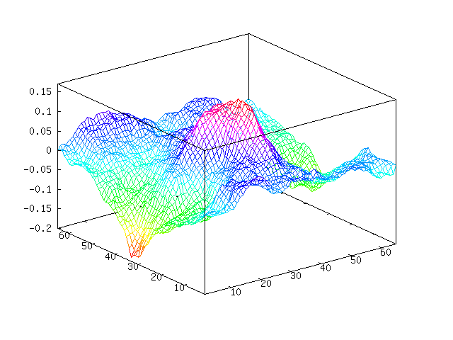
You can see we have a sort of mountain going on in the middle. Here is
the “plasma fractal” view of our noise.

These were generated using this Octave code. I believe that this is
both the fastest and most concise way to do this in Octave. You can
see we are throwing away a lot of random values that we pulled, but at
the same time avoiding loops. You will need at least version 2.9 of
Octave because, as far as I know, Octave 2.1 doesn’t have interp2.
And, unfortunately, interp2 is much slower than it probably could
be.
function m = diamond_square (m, i, c)
  if isempty (m)
    m = zeros (2);
  end

  for k = 1:i
    m = interp2 (m, 1);

    %% Define points we want to randomize
    gridmap = ones (size (m));
    gridmap(1:2:end, 1:2:end) = 0;
    gridmap = find(gridmap);       % Makes Octave happy

    %% Define random values to be added
    randmap = c * randn (size (m));

    m(gridmap) += randmap(gridmap);

    c = c / 2;
  end
end
Something of note here compared to other implementations of
diamond-square, my code above adds Gaussian noise (with Octave’s
randn) rather than uniform noise. The scaling variable c is
actually adjusting the standard deviation of our noise and not the
limits of the noise. I imagine this makes the terrain more natural, as
Gaussian noise tends to approximate real noise well.
The first argument provides a base terrain to work from. With this you
can define a mountain, islands, hillside, etc. When an empty matrix is
provided, the terrain will be grown from flat ground. The second
argument decides how many iterations we are going to run. The above
example performs 6 iterations on flat terrain. The last argument
decides how dramatic the terrain is, which doesn’t have much meaning
when starting from flat terrain. The example above was produced with
two calls like this (one for each image),
octave> mesh(m=diamond_square([], 6, 0.1))
octave> imagesc(m); colormap(gray);
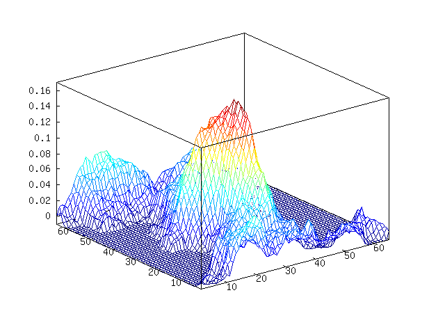
We can add some water, or perhaps lava or something, by choosing a
water height and chopping off everything below it. I will choose
-0.1 as our water level.
octave> w = m;
octave> w(w < -0.01) = -0.01;
octave> mesh(w)
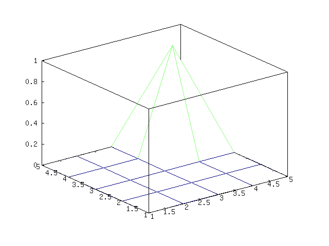
Here is an example of providing some base terrain. Let’s put a
mountain in the corner of the map,
octave> a = [0 0 0 0 0; 0 0 0 0 0; 0 0 0 0 0; 0 0 0 1 0; 0 0 0 0 0]
octave> mesh (b = diamond_square (a, 4, 0.15))
Becomes,
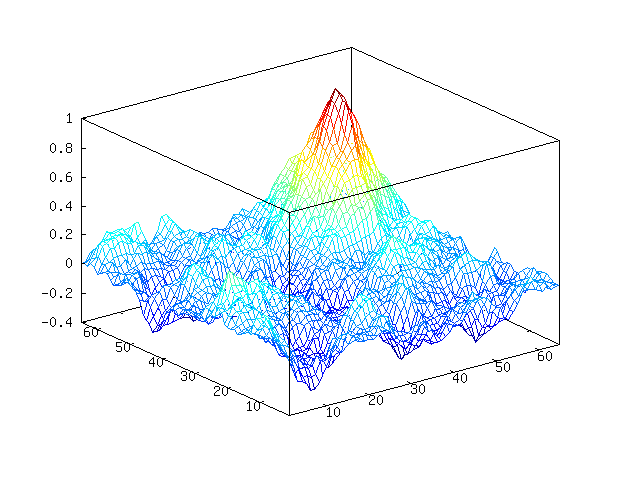
Octave-Forge has a surf function that should make this look nicer,
but it doesn’t. If we want to render this to make it look nice, we
will need another program to do it. Let’s do that another time.
Update May 2012: I have come to realize the below is not
Perlin noise. It is actually
fractional Brownian motion, which is a bit simpler than
Perlin noise.
Another way to make noise is fractional Brownian motion
(FBM). Generally, this noise will be better and more useful than
diamond-square noise (examples later). I personally like this person’s
(mislabeled) approach: FPM Noise. It is easy to implement and
understand, though it doesn’t have the all advantages you get
from generating Perlin noise.
If you don’t feel like clicking through and see the nice introduction
to FBM noise there, here is the idea of this approach: we create
different frequencies of noise and mix them all together, giving more
weight to lower frequency noise than high frequency noise. Below, you
can see that I generated (Gaussian) noise in different frequencies,
smoothing by spline interpolation. Then we add this all together to
get our final FBM noise.


Here is the Octave code I am using to generate FBM noise,
function s = fbm (m)
  s = zeros(m);    % output image
  w = m;           % width of current layer
  i = 0;           % iterations
  while w > 3
    i = i + 1;
    d = interp2(randn(w), i-1, "spline");
    s = s + i * d(1:m, 1:m);
    w -= ceil(w/2 - 1);
  end
end
The first and only argument gives the side length of the image you
want to generate - it only generates square images. This is an
extremely simple approach, as there are no parameters to adjust to
define the nature of the noise you want to generate. Fortunately, what
I am going to try next works fine without these parameters (or with
the default, hard-coded parameters if you wish).
Continuing with using some ideas from Hugo Elias, I am going
to use this noise to attempt to create some realistic looking clouds.
First, we will generate some noise. Let’s generate some FBM noise,
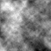
Now, this doesn’t look too much like clouds. To get clouds, we can
apply an exponential function to the data and set anything below 0 to
0 (contrast stretching). If we scale our noise between 0 and 1, the
function will look like this,
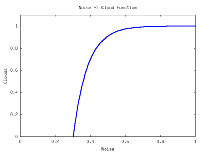
To adjust the clouds, we can move this function left and right across
the x-axis. We can adjust the “time constant” of the function to
change the sharpness of the clouds. Here is the function I wrote to
convert the diamond-square or FBM noise into cloud cover. The output
is scaled between 0 and 255 to aid in image output.
function a = get_clouds (a)
  %% Scale a between 0 and 1
  a = a - min(a(:));
  a = a / max(a(:));

  %% Parameters
  density = 0.5;
  sharpness = 0.1;

  a = 1 - e.^(-(a - density) * sharpness);
  a(a < 0) = 0;

  %% Scale between 0 to 255 and quantize
  a = a / max(a(:));
  a = round(a * 255);
end
Now run this on our noise,
octave> c = get_clouds(n);
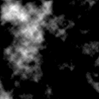
Well, that looks a bit more like cloud cover. We just need to apply a
colormap to this. I wrote this colormap function for this purpose,
function c = cloud_cmap ()
  c = [0.25 0.25 1];
  for i = 2:256
    c(i, :) = (i-2)/256 * (1 - c(2, :)) + c(2, :);
  end
end
Apply the colormap,
octave> imwrite("clouds.png", c+1, cloud_cmap)
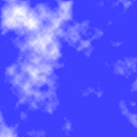
Wow, that looks pretty good now. We could improve this by fading to
transparent rather than blue. Then do a projective transformation on
the clouds and lay them over top a blue gradient. You could do this
with image editing software such as the Gimp, or you can
continue to use Octave like I did at the end of this post.
So, in about 30 lines of Octave (including code on the interactive
command line) code we could generate some kind-of realistic looking
clouds. Here, I will use the cloud demo to show one particular
advantage of FBM noise over diamond-square (or at least my
implementation). Here are some diamond-square clouds,
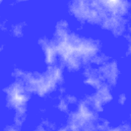
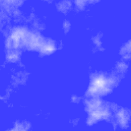
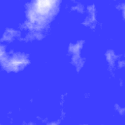
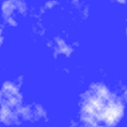
And here are some FBM clouds, which I think look a bit better,
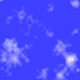
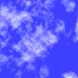
Notice the straight lines in the diamond-square clouds? You can see it
right in the middle of the first image. This comes from the way that
the 2-dimensional interpolation stretches the noise in the vertical
and horizontal directions, drawing these lines out. This may only be
apparent in my implementation, as I am probably missing the “diamond”
part of the algorithm. Oh well.
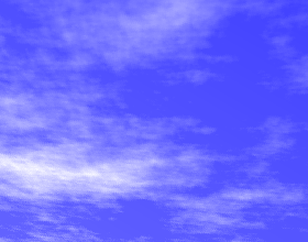
Anyway, to take the clouds a bit further, you can use Octave’s
imperspectivewarp to apply a perspective transformation to the cloud
images. I put some code together that does this transformation as well
as adds a gradient,
function i = pers_clouds (n)
  w = size(n, 1);
  c = get_clouds (n);
  t = -pi/32;
  P = [cos(t) sin(t) 0; -sin(t) cos(t) 0; 0.001 0.002 1];

  %% Perspective transformation
  pc = imperspectivewarp (c/255, P, "cubic");
  pw = size(pc, 1);
  ph = size(pc, 2);

  %% Create and combine background gradient
  [dump back] = meshgrid(1:ph, 1:pw);
  i = pc * 4 * pw + back;

  %% Fit between 0 to 255 for image
  i = i - min (i(:));
  i = round (i / max (i(:)) * 255);
  i(isnan(i)) = 0;
end
Provide either FBM noise or diamond-square noise and it will return an
image that you can write out to a file,
octave> n = fbm (1000);
octave> imwrite ("clouds.png", pers_clouds(n) + 1, cloud_cmap)
After cropping the image with something like kolourpaint (as I
did below), you get,

Update: Sebastian Schaetz used my code above in a
random map generator. Check it out.